Amplifier Design for Maximum Gain
Single-Stage Microwave Transistor Amplifier Design and Maximum Gain
1. Single-Stage Microwave Transistor Amplifier
A single-stage microwave transistor amplifier is a fundamental microwave circuit used to increase the power level of an input RF signal while providing the required gain at a selected operating frequency. Unlike low-frequency amplifier design, microwave transistor amplifiers are strongly influenced by transmission-line effects, complex impedances, reflection coefficients, and the scattering parameters of the transistor. Therefore, the design of a microwave amplifier requires careful control of the signal entering the transistor as well as the signal delivered from the transistor to the load.
A typical single-stage microwave transistor amplifier consists of a source, an input matching network, the microwave transistor, an output matching network, and the load. The transistor is characterized by its four scattering parameters \(S_{11}\), \(S_{12}\), \(S_{21}\), and \(S_{22}\), which describe the input reflection, reverse transmission, forward transmission, and output reflection characteristics, respectively. At microwave frequencies, these parameters provide a convenient way to analyze the transistor without requiring direct measurement of conventional open-circuit or short-circuit parameters.
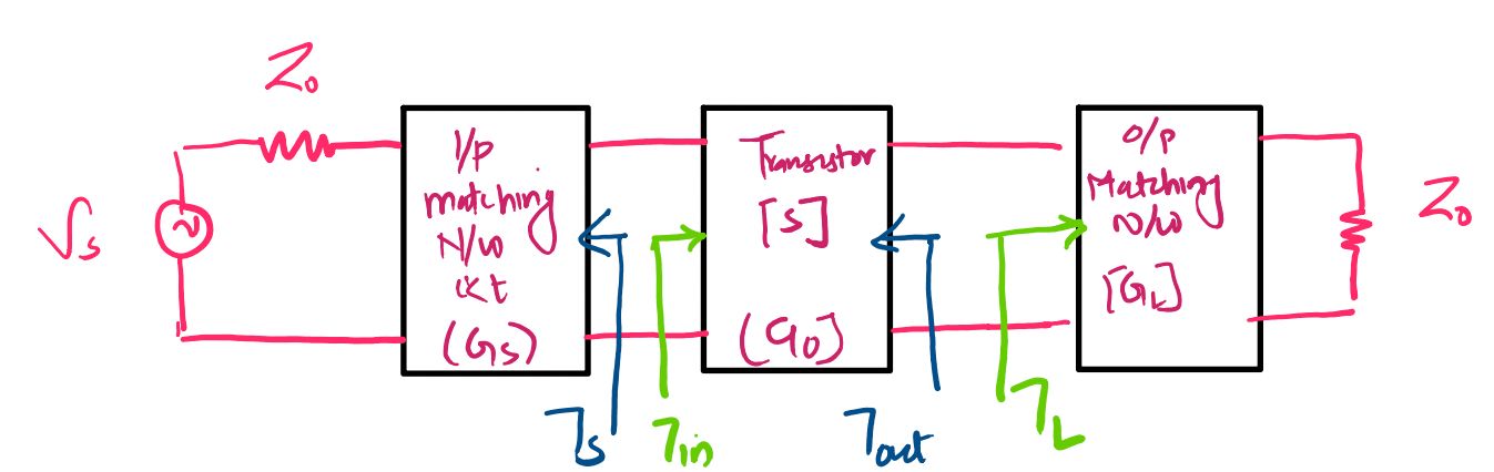
The input and output matching networks are important because the transistor does not generally present the impedance required for maximum power transfer from the source or to the load. The input matching network transforms the source impedance into an appropriate impedance at the transistor input, while the output matching network transforms the transistor output impedance into an appropriate load impedance. In terms of reflection coefficients, these networks establish suitable values of the source reflection coefficient \(\Gamma_S\) and load reflection coefficient \(\Gamma_L\).
The matching networks also determine how effectively the available signal power is transferred into and out of the transistor. Consequently, maximum-gain amplifier design is not simply a matter of selecting a transistor with a large \(S_{21}\). The source and load must be selected appropriately, and the stability of the transistor must also be considered. A matching condition that theoretically provides high gain may not be physically realizable if it requires a source or load reflection coefficient outside the passive region, or if it places the amplifier in an unstable operating condition.
The design procedure therefore begins by determining the transistor's scattering parameters and stability characteristics, followed by determining the appropriate source and load reflection coefficients. For a unilateral transistor, the input and output matching conditions can be treated independently because reverse transmission is negligible. For a bilateral transistor, however, the source and load matching conditions are coupled through the reverse transmission parameter \(S_{12}\), requiring a simultaneous solution.
2. Maximum Gain Condition
The objective of maximum-gain design is to select the source and load conditions so that the transistor transfers as much of the available input power to the load as possible. The quantity commonly used to describe the overall power transfer through a microwave amplifier is the transducer power gain, \(G_T\). It represents the ratio of the power delivered to the load to the power available from the source.
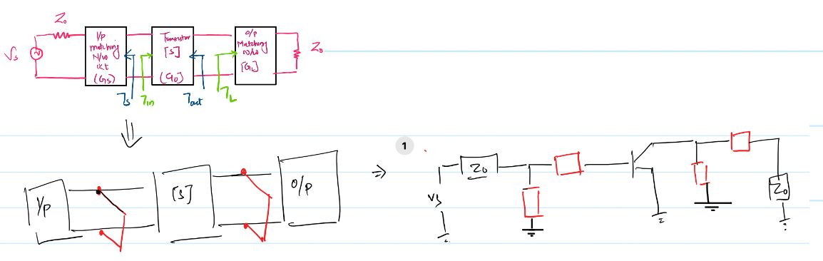
For a given transistor and operating frequency, the transducer gain depends on both the source reflection coefficient \(\Gamma_S\) and the load reflection coefficient \(\Gamma_L\). Maximum power transfer occurs when the source and load networks satisfy the appropriate conjugate-matching conditions. At the transistor input, the source must be conjugately matched to the input reflection coefficient. Similarly, at the transistor output, the load must be conjugately matched to the output reflection coefficient.
The input conjugate-matching condition is written as
\[ \Gamma_{in}=\Gamma_S^{*} \]
and the output conjugate-matching condition is
\[ \Gamma_{out}=\Gamma_L^{*} \]
Taking the complex conjugate of these relationships gives the equivalent conditions
\[ \Gamma_S=\Gamma_{in}^{*} \]
\[ \Gamma_L=\Gamma_{out}^{*} \]
These equations form the fundamental basis of simultaneous conjugate matching. They indicate that the reflection coefficient presented by the source should be the complex conjugate of the reflection coefficient looking into the transistor input, while the reflection coefficient presented by the load should be the complex conjugate of the reflection coefficient looking toward the transistor output.
For a microwave transistor, the input and output reflection coefficients are determined from the transistor's scattering parameters and the termination at the opposite port. Therefore, the actual matching conditions depend on whether the transistor is unilateral or bilateral. This distinction becomes particularly important when \(S_{12}\) is not negligible, because the load then affects the input reflection coefficient and the source affects the output reflection coefficient.
3. Physical Meaning of Simultaneous Conjugate Matching
Simultaneous conjugate matching means satisfying the input and output conjugate-matching conditions at the same time. The purpose is to maximize power transfer at both sides of the transistor: the input matching network delivers the maximum available power from the source to the transistor, while the output matching network allows the transistor to deliver the maximum available power to the load.
The word simultaneous is important because the two matching conditions are not always independent. In an ideal unilateral transistor, the reverse transmission parameter is zero, \(S_{12}=0\). Under this condition, the output termination does not influence the input reflection coefficient, and the source termination does not influence the output reflection coefficient. The input and output matching networks can therefore be designed independently.
For a bilateral transistor, \(S_{12}\neq0\), so a change in the load reflection coefficient can change the input reflection coefficient, while a change in the source reflection coefficient can change the output reflection coefficient. Consequently, the two conjugate-matching conditions become coupled equations. The optimum values of \(\Gamma_S\) and \(\Gamma_L\) must then be obtained simultaneously rather than by independently setting each one equal to the conjugate of \(S_{11}\) or \(S_{22}\).
This coupling is the reason that maximum-gain design for a bilateral microwave transistor requires a more detailed mathematical treatment. The simultaneous matching equations can be rearranged to produce quadratic equations for the optimum source and load reflection coefficients. These equations, together with the transistor's stability conditions, determine whether the desired maximum-gain matching condition can be physically realized.
4. Maximum Transducer Power Gain
The transducer power gain of a two-port microwave transistor can be expressed in terms of its scattering parameters and the source and load reflection coefficients. For the standard single-stage amplifier configuration, the transducer gain is
\[ G_T= \frac{1-|\Gamma_S|^2} {|1-S_{11}\Gamma_S|^2} |S_{21}|^2 \frac{1-|\Gamma_L|^2} {|1-S_{22}\Gamma_L|^2} \]
This expression can be understood as the product of three important effects. The first factor
\[ \frac{1-|\Gamma_S|^2} {|1-S_{11}\Gamma_S|^2} \]
describes the power transfer at the input side of the transistor. It depends on the source reflection coefficient \(\Gamma_S\) and the transistor input scattering parameter \(S_{11}\). The factor reaches its maximum when the source is conjugately matched to the transistor input.
The middle factor
\[ |S_{21}|^2 \]
represents the forward power transmission capability of the transistor. Since \(S_{21}\) is a voltage-wave transmission coefficient, its squared magnitude represents the corresponding power-wave transmission factor under the standard reference-impedance conditions.
The final factor
\[ \frac{1-|\Gamma_L|^2} {|1-S_{22}\Gamma_L|^2} \]
represents the power transfer from the transistor output to the load. It depends on the load reflection coefficient \(\Gamma_L\) and the transistor output scattering parameter \(S_{22}\). This factor is maximized when the load is conjugately matched to the transistor output.
Therefore, maximum transducer gain is obtained by selecting the source and load reflection coefficients so that the simultaneous conjugate-matching conditions are satisfied:
\[ \Gamma_S=\Gamma_{in}^{*} \]
\[ \Gamma_L=\Gamma_{out}^{*} \]
For a unilateral transistor, these conditions lead directly to independent source and load matching. For a bilateral transistor, however, \(\Gamma_{in}\) depends on \(\Gamma_L\) and \(\Gamma_{out}\) depends on \(\Gamma_S\). The resulting coupled equations are the starting point for the detailed derivation of the optimum source and load reflection coefficients in the next part.
Bilateral Transistor and Simultaneous Conjugate Matching
2.1 Bilateral Transistor Behavior
A microwave transistor is called a bilateral transistor when signal transmission occurs in both directions between its input and output ports. In terms of scattering parameters, this behavior is represented by a nonzero reverse transmission coefficient:
\[ S_{12}\neq0 \]
Here, \(S_{12}\) represents the reverse transmission from port 2 to port 1, while \(S_{21}\) represents the forward transmission from port 1 to port 2. When \(S_{12}\neq0\), a signal or reflection at the output side can propagate back toward the input side. As a result, the input characteristics of the transistor are affected by the load connected to port 2. Similarly, a change in the source termination at port 1 affects the output characteristics.
This behavior can be obtained directly from the scattering-parameter equations. For a two-port transistor, the output waves are related to the incident waves by
\[ b_1=S_{11}a_1+S_{12}a_2 \]
\[ b_2=S_{21}a_1+S_{22}a_2 \]
At the output port, the load reflection coefficient is defined as
\[ \Gamma_L=\frac{a_2}{b_2} \]
Therefore,
\[ a_2=\Gamma_L b_2 \]
Substituting the expression for \(b_2\),
\[ a_2 = \Gamma_L \left( S_{21}a_1+S_{22}a_2 \right) \]
Expanding the right-hand side gives
\[ a_2 = S_{21}\Gamma_L a_1 + S_{22}\Gamma_L a_2 \]
Collecting the terms containing \(a_2\),
\[ a_2-S_{22}\Gamma_L a_2 = S_{21}\Gamma_L a_1 \]
\[ a_2(1-S_{22}\Gamma_L) = S_{21}\Gamma_L a_1 \]
Hence,
\[ \frac{a_2}{a_1} = \frac{S_{21}\Gamma_L} {1-S_{22}\Gamma_L} \]
Now substitute this result into the input-port equation:
\[ b_1 = S_{11}a_1+S_{12}a_2 \]
\[ b_1 = S_{11}a_1 + S_{12} \left( \frac{S_{21}\Gamma_L} {1-S_{22}\Gamma_L} \right)a_1 \]
Dividing by \(a_1\), the input reflection coefficient becomes
\[ \Gamma_{in} = \frac{b_1}{a_1} = S_{11} + \frac{S_{12}S_{21}\Gamma_L} {1-S_{22}\Gamma_L} \]
This equation clearly shows the effect of bilateral operation. Because \(S_{12}\neq0\), the input reflection coefficient \(\Gamma_{in}\) depends on the load reflection coefficient \(\Gamma_L\). Therefore, changing the load matching network changes the input matching condition.
The same procedure can be applied to the output side. At the input port, the source reflection coefficient is defined as
\[ \Gamma_S=\frac{a_1}{b_1} \]
Therefore,
\[ a_1=\Gamma_S b_1 \]
Substituting the expression for \(b_1\),
\[ a_1 = \Gamma_S \left( S_{11}a_1+S_{12}a_2 \right) \]
Expanding and collecting the terms containing \(a_1\),
\[ a_1 = S_{11}\Gamma_S a_1 + S_{12}\Gamma_S a_2 \]
\[ a_1-S_{11}\Gamma_S a_1 = S_{12}\Gamma_S a_2 \]
\[ a_1(1-S_{11}\Gamma_S) = S_{12}\Gamma_S a_2 \]
Hence,
\[ \frac{a_1}{a_2} = \frac{S_{12}\Gamma_S} {1-S_{11}\Gamma_S} \]
Substituting this relationship into the output-port equation
\[ b_2=S_{21}a_1+S_{22}a_2 \]
gives
\[ b_2 = S_{21} \left( \frac{S_{12}\Gamma_S} {1-S_{11}\Gamma_S} \right)a_2 + S_{22}a_2 \]
Dividing by \(a_2\), the output reflection coefficient becomes
\[ \Gamma_{out} = \frac{b_2}{a_2} = S_{22} + \frac{S_{12}S_{21}\Gamma_S} {1-S_{11}\Gamma_S} \]
Thus, \(\Gamma_{out}\) depends on \(\Gamma_S\) whenever \(S_{12}\neq0\). The bilateral transistor therefore creates a two-way coupling: the load affects the input reflection coefficient, and the source affects the output reflection coefficient.
2.2 Simultaneous Matching Equations
For maximum power transfer, the source and load must satisfy conjugate-matching conditions. At the input, the source reflection coefficient must be the complex conjugate of the input reflection coefficient:
\[ \Gamma_S=\Gamma_{in}^{*} \]
Equivalently,
\[ \Gamma_S^{*}=\Gamma_{in} \]
Using the previously derived expression for \(\Gamma_{in}\),
\[ \Gamma_S^{*} = S_{11} + \frac{S_{12}S_{21}\Gamma_L} {1-S_{22}\Gamma_L} \]
Similarly, maximum power transfer at the output requires
\[ \Gamma_L=\Gamma_{out}^{*} \]
or equivalently,
\[ \Gamma_L^{*}=\Gamma_{out} \]
Using the derived expression for \(\Gamma_{out}\),
\[ \Gamma_L^{*} = S_{22} + \frac{S_{12}S_{21}\Gamma_S} {1-S_{11}\Gamma_S} \]
Therefore, the two simultaneous conjugate-matching equations are
\[ \boxed{ \Gamma_S^{*} = S_{11} + \frac{S_{12}S_{21}\Gamma_L} {1-S_{22}\Gamma_L} } \]
\[ \boxed{ \Gamma_L^{*} = S_{22} + \frac{S_{12}S_{21}\Gamma_S} {1-S_{11}\Gamma_S} } \]
These two equations must be satisfied at the same time. Unlike the unilateral case, the first equation contains \(\Gamma_L\), while the second contains \(\Gamma_S\). Consequently, neither reflection coefficient can generally be determined independently.
To derive an equation containing only \(\Gamma_S\), the second matching equation is first rearranged. Starting with
\[ \Gamma_L^{*} = S_{22} + \frac{S_{12}S_{21}\Gamma_S} {1-S_{11}\Gamma_S} \]
put the terms over a common denominator:
\[ \Gamma_L^{*} = \frac{ S_{22}(1-S_{11}\Gamma_S) + S_{12}S_{21}\Gamma_S } {1-S_{11}\Gamma_S} \]
Expanding the numerator gives
\[ \Gamma_L^{*} = \frac{ S_{22} - S_{11}S_{22}\Gamma_S + S_{12}S_{21}\Gamma_S } {1-S_{11}\Gamma_S} \]
Grouping the terms containing \(\Gamma_S\),
\[ \Gamma_L^{*} = \frac{ S_{22} - \left( S_{11}S_{22}-S_{12}S_{21} \right)\Gamma_S } {1-S_{11}\Gamma_S} \]
This naturally introduces the determinant of the scattering matrix.
2.3 Determinant of the S-Matrix
The determinant of the two-port scattering matrix is defined as
\[ \Delta = S_{11}S_{22} - S_{12}S_{21} \]
Using this definition,
\[ S_{11}S_{22}-S_{12}S_{21}=\Delta \]
Therefore, the numerator obtained from the output matching equation becomes
\[ S_{22}-\Delta\Gamma_S \]
and the output matching equation can be written as
\[ \boxed{ \Gamma_L^{*} = \frac{ S_{22}-\Delta\Gamma_S } { 1-S_{11}\Gamma_S } } \]
This form is particularly useful because it expresses \(\Gamma_L^{*}\) entirely in terms of \(\Gamma_S\) and the transistor scattering parameters. It can therefore be substituted into the first simultaneous matching equation to eliminate \(\Gamma_L\).
To perform this elimination, first take the complex conjugate of the source matching equation:
\[ \Gamma_S = S_{11}^{*} + \frac{ S_{12}^{*}S_{21}^{*} }{ \frac{1}{\Gamma_L^{*}}-S_{22}^{*} } \]
Now substitute
\[ \Gamma_L^{*} = \frac{ S_{22}-\Delta\Gamma_S } { 1-S_{11}\Gamma_S } \]
into this equation. This gives
\[ \Gamma_S = S_{11}^{*} + \frac{ S_{12}^{*}S_{21}^{*} }{ \frac{1}{ \frac{S_{22}-\Delta\Gamma_S} {1-S_{11}\Gamma_S} } -S_{22}^{*} } \]
The reciprocal of the fraction in the denominator is
\[ \frac{1}{ \frac{S_{22}-\Delta\Gamma_S} {1-S_{11}\Gamma_S} } = \frac{1-S_{11}\Gamma_S} {S_{22}-\Delta\Gamma_S} \]
Therefore, the equation becomes
\[ \Gamma_S = S_{11}^{*} + \frac{ S_{12}^{*}S_{21}^{*} }{ \frac{1-S_{11}\Gamma_S} {S_{22}-\Delta\Gamma_S} -S_{22}^{*} } \]
Putting the denominator over a common denominator gives
\[ \Gamma_S = S_{11}^{*} + \frac{ S_{12}^{*}S_{21}^{*} }{ \frac{ 1-S_{11}\Gamma_S - S_{22}^{*}(S_{22}-\Delta\Gamma_S) } { S_{22}-\Delta\Gamma_S } } \]
Expanding the numerator of this new denominator,
\[ 1-S_{11}\Gamma_S - S_{22}S_{22}^{*} + \Delta\Gamma_S S_{22}^{*} \]
Since
\[ S_{22}S_{22}^{*}=|S_{22}|^2 \]
the expression becomes
\[ 1-S_{11}\Gamma_S - |S_{22}|^2 + \Delta\Gamma_S S_{22}^{*} \]
Hence,
\[ \Gamma_S = S_{11}^{*} + \frac{ S_{12}^{*}S_{21}^{*} (S_{22}-\Delta\Gamma_S) } { 1-S_{11}\Gamma_S -|S_{22}|^2 +\Delta\Gamma_S S_{22}^{*} } \]
This is the required single equation in \(\Gamma_S\). Expanding and collecting its terms leads to the quadratic equation for the optimum source reflection coefficient, which is derived completely in the next part.
2.4 Coupling of Source and Load Matching
The mathematical coupling between the source and load matching conditions can now be seen directly from the two simultaneous equations:
\[ \Gamma_S^{*} = S_{11} + \frac{S_{12}S_{21}\Gamma_L} {1-S_{22}\Gamma_L} \]
\[ \Gamma_L^{*} = S_{22} + \frac{S_{12}S_{21}\Gamma_S} {1-S_{11}\Gamma_S} \]
The first equation shows that \(\Gamma_S\) depends on \(\Gamma_L\), while the second shows that \(\Gamma_L\) depends on \(\Gamma_S\). This mutual dependence is a direct consequence of the nonzero reverse transmission parameter \(S_{12}\).
Therefore, independently selecting
\[ \Gamma_S=S_{11}^{*} \]
and
\[ \Gamma_L=S_{22}^{*} \]
is not generally valid for a bilateral transistor. Those expressions become the appropriate conjugate-matching conditions only under the unilateral approximation \(S_{12}=0\). When \(S_{12}\neq0\), the additional coupling terms involving \(S_{12}S_{21}\) must be included.
The determinant \(\Delta\) provides a convenient way to handle this coupling mathematically. By expressing \(\Gamma_L^{*}\) in terms of \(\Gamma_S\), the two simultaneous equations can be reduced to a single quadratic equation in \(\Gamma_S\). Once the physically realizable solution for \(\Gamma_S\) is obtained, the corresponding \(\Gamma_L\) can be determined from the matching relationship.
Thus, the bilateral amplifier design problem becomes a mathematical problem of solving coupled conjugate-matching equations and then selecting the physically meaningful source and load reflection coefficients. The complete expansion of the single-\(\Gamma_S\) equation, formation of the quadratic equation, definition of the auxiliary parameters \(B_1\) and \(C_1\), and solution for the optimum reflection coefficients are developed in the next part.
Detailed Derivation of Optimum Source and Load Reflection Coefficients
3.1 Rearranging the Source Matching Equation
For a bilateral microwave transistor, the optimum source and load reflection coefficients are obtained by solving the simultaneous conjugate-matching equations. The derivation begins with the source matching equation after taking the complex conjugate of the input matching relationship:
\[ \Gamma_S = S_{11}^{*} + \frac{S_{12}^{*}S_{21}^{*}} {\dfrac{1}{\Gamma_L^{*}}-S_{22}^{*}} \]
From the output matching equation, the load reflection coefficient can be expressed in terms of the source reflection coefficient. Starting with
\[ \Gamma_L^{*} = S_{22} + \frac{S_{12}S_{21}\Gamma_S} {1-S_{11}\Gamma_S} \]
putting the terms over a common denominator gives
\[ \Gamma_L^{*} = \frac{ S_{22}(1-S_{11}\Gamma_S) + S_{12}S_{21}\Gamma_S } { 1-S_{11}\Gamma_S } \]
Expanding the numerator,
\[ \Gamma_L^{*} = \frac{ S_{22} - S_{11}S_{22}\Gamma_S + S_{12}S_{21}\Gamma_S } { 1-S_{11}\Gamma_S } \]
Using the determinant of the scattering matrix,
\[ \Delta = S_{11}S_{22} - S_{12}S_{21} \]
the terms multiplying \(\Gamma_S\) can be written as
\[ S_{11}S_{22}-S_{12}S_{21}=\Delta \]
Therefore,
\[ \boxed{ \Gamma_L^{*} = \frac{ S_{22}-\Delta\Gamma_S } { 1-S_{11}\Gamma_S } } \]
This expression is now substituted into the rearranged source matching equation. Thus,
\[ \Gamma_S = S_{11}^{*} + \frac{ S_{12}^{*}S_{21}^{*} }{ \frac{1}{\Gamma_L^{*}}-S_{22}^{*} } \]
becomes
\[ \Gamma_S = S_{11}^{*} + \frac{ S_{12}^{*}S_{21}^{*} }{ \frac{1}{ \frac{S_{22}-\Delta\Gamma_S} {1-S_{11}\Gamma_S} } -S_{22}^{*} } \]
Taking the reciprocal of the fraction in the denominator gives
\[ \Gamma_S = S_{11}^{*} + \frac{ S_{12}^{*}S_{21}^{*} }{ \frac{1-S_{11}\Gamma_S} {S_{22}-\Delta\Gamma_S} -S_{22}^{*} } \]
Next, combine the two terms in the denominator over a common denominator:
\[ \frac{1-S_{11}\Gamma_S} {S_{22}-\Delta\Gamma_S} -S_{22}^{*} = \frac{ 1-S_{11}\Gamma_S - S_{22}^{*}(S_{22}-\Delta\Gamma_S) } { S_{22}-\Delta\Gamma_S } \]
Expanding the numerator gives
\[ 1-S_{11}\Gamma_S - S_{22}S_{22}^{*} + \Delta\Gamma_S S_{22}^{*} \]
Since
\[ S_{22}S_{22}^{*}=|S_{22}|^2 \]
the denominator becomes
\[ 1-S_{11}\Gamma_S -|S_{22}|^2 +\Delta\Gamma_S S_{22}^{*} \]
Therefore,
\[ \Gamma_S = S_{11}^{*} + \frac{ S_{12}^{*}S_{21}^{*} (S_{22}-\Delta\Gamma_S) } { 1-S_{11}\Gamma_S -|S_{22}|^2 +\Delta\Gamma_S S_{22}^{*} } \]
The equation is now in a form containing only \(\Gamma_S\). The next step is to eliminate the fraction by cross multiplication.
3.2 Formation of the Quadratic Equation for \(\Gamma_S\)
Starting from
\[ \Gamma_S = S_{11}^{*} + \frac{ S_{12}^{*}S_{21}^{*} (S_{22}-\Delta\Gamma_S) } { 1-S_{11}\Gamma_S -|S_{22}|^2 +\Delta\Gamma_S S_{22}^{*} } \]
multiply both sides by the denominator:
\[ \Gamma_S \left[ 1-S_{11}\Gamma_S -|S_{22}|^2 +\Delta\Gamma_S S_{22}^{*} \right] \]
\[ = S_{11}^{*} \left[ 1-S_{11}\Gamma_S -|S_{22}|^2 +\Delta\Gamma_S S_{22}^{*} \right] + S_{12}^{*}S_{21}^{*} (S_{22}-\Delta\Gamma_S) \]
Expanding the left-hand side gives
\[ \Gamma_S - S_{11}\Gamma_S^2 - |S_{22}|^2\Gamma_S + \Delta S_{22}^{*}\Gamma_S^2 \]
The right-hand side becomes
\[ S_{11}^{*} - |S_{11}|^2\Gamma_S - S_{11}^{*}|S_{22}|^2 + S_{11}^{*}\Delta S_{22}^{*}\Gamma_S + S_{12}^{*}S_{21}^{*}S_{22} - S_{12}^{*}S_{21}^{*}\Delta\Gamma_S \]
Move all terms to the left-hand side and collect the terms containing \(\Gamma_S^2\), \(\Gamma_S\), and the constant terms. The coefficient of \(\Gamma_S^2\) is
\[ -S_{11}+\Delta S_{22}^{*} \]
Multiplying the complete equation by \(-1\), the quadratic coefficient becomes
\[ S_{11}-\Delta S_{22}^{*} \]
For the constant terms, we obtain
\[ S_{11}^{*} - S_{11}^{*}|S_{22}|^2 + S_{12}^{*}S_{21}^{*}S_{22} \]
Using
\[ \Delta^{*} = S_{11}^{*}S_{22}^{*} - S_{12}^{*}S_{21}^{*} \]
we can write
\[ \Delta^{*}S_{22} = S_{11}^{*}|S_{22}|^2 - S_{12}^{*}S_{21}^{*}S_{22} \]
Therefore, the constant terms reduce to
\[ S_{11}^{*}-\Delta^{*}S_{22} \]
The coefficient of \(\Gamma_S\) can be simplified using the determinant identity
\[ \Delta = S_{11}S_{22}-S_{12}S_{21} \]
and its complex conjugate
\[ \Delta^{*} = S_{11}^{*}S_{22}^{*} - S_{12}^{*}S_{21}^{*} \]
so that
\[ |\Delta|^2 = \Delta\Delta^{*} \]
and consequently
\[ \Delta S_{11}^{*}S_{22}^{*} - \Delta S_{12}^{*}S_{21}^{*} = |\Delta|^2 \]
After collecting and simplifying all terms, the resulting quadratic equation is
\[ \boxed{ \Gamma_S^2 (S_{11}-\Delta S_{22}^{*}) + \Gamma_S \left[ -1-|S_{11}|^2+|S_{22}|^2+|\Delta|^2 \right] + (S_{11}^{*}-\Delta^{*}S_{22}) = 0 } \]
The middle coefficient is important because it must be consistent with the standard definitions of \(B_1\) and \(C_1\) used for the optimum source reflection coefficient. Defining
\[ B_1 = 1+|S_{11}|^2-|S_{22}|^2-|\Delta|^2 \]
gives
\[ -B_1 = -1-|S_{11}|^2+|S_{22}|^2+|\Delta|^2 \]
Therefore, the quadratic can be written compactly as
\[ C_1\Gamma_S^2-B_1\Gamma_S+C_1^{*}=0 \]
3.3 Defining \(B_1\) and \(C_1\)
To make the quadratic equation easier to solve, define the auxiliary quantity
\[ \boxed{ B_1 = 1+|S_{11}|^2-|S_{22}|^2-|\Delta|^2 } \]
and
\[ \boxed{ C_1 = S_{11}-\Delta S_{22}^{*} } \]
The complex conjugate of \(C_1\) is
\[ C_1^{*} = S_{11}^{*}-\Delta^{*}S_{22} \]
Thus, the expanded quadratic becomes
\[ C_1\Gamma_S^2-B_1\Gamma_S+C_1^{*}=0 \]
This form is convenient because the first and third coefficients are complex conjugates of one another. The equation can now be solved directly using the quadratic formula.
3.4 Solution for the Optimum Source Reflection Coefficient
For a quadratic equation of the form
\[ a x^2+b x+c=0 \]
the solutions are
\[ x= \frac{-b\pm\sqrt{b^2-4ac}}{2a} \]
Comparing this standard form with
\[ C_1\Gamma_S^2-B_1\Gamma_S+C_1^{*}=0 \]
gives
\[ a=C_1 \]
\[ b=-B_1 \]
\[ c=C_1^{*} \]
Substituting these values into the quadratic formula gives
\[ \Gamma_S = \frac{ B_1 \pm \sqrt{ B_1^2-4C_1C_1^{*} } } {2C_1} \]
Since
\[ C_1C_1^{*}=|C_1|^2 \]
the optimum source reflection coefficient is therefore
\[ \boxed{ \Gamma_S = \frac{ B_1 \pm \sqrt{B_1^2-4|C_1|^2} } {2C_1} } \]
The plus and minus signs produce two mathematical roots. Both roots satisfy the quadratic equation mathematically, but they do not necessarily represent physically realizable source terminations. Each root must therefore be examined by checking its magnitude and the stability conditions of the transistor.
3.5 Derivation and Solution for the Optimum Load Reflection Coefficient
The optimum load reflection coefficient can be obtained by following the same derivation from the output side. The roles of the input and output ports are interchanged, resulting in a quadratic equation of the corresponding form:
\[ C_2\Gamma_L^2-B_2\Gamma_L+C_2^{*}=0 \]
where
\[ \boxed{ B_2 = 1+|S_{22}|^2-|S_{11}|^2-|\Delta|^2 } \]
and
\[ \boxed{ C_2 = S_{22}-\Delta S_{11}^{*} } \]
The complex conjugate of \(C_2\) is
\[ C_2^{*} = S_{22}^{*}-\Delta^{*}S_{11} \]
Applying the quadratic formula to
\[ C_2\Gamma_L^2-B_2\Gamma_L+C_2^{*}=0 \]
gives
\[ \Gamma_L = \frac{ B_2 \pm \sqrt{ B_2^2-4C_2C_2^{*} } } {2C_2} \]
Since
\[ C_2C_2^{*}=|C_2|^2 \]
the optimum load reflection coefficient becomes
\[ \boxed{ \Gamma_L = \frac{ B_2 \pm \sqrt{B_2^2-4|C_2|^2} } {2C_2} } \]
As with the source reflection coefficient, the two signs produce two mathematical solutions. The appropriate solution must be selected using the physical requirements of the source and load networks and the stability characteristics of the transistor.
3.6 Selection of the Physically Realizable Solution
The quadratic equations can produce two mathematical roots for both \(\Gamma_S\) and \(\Gamma_L\). However, a mathematical root is not automatically a realizable microwave termination. For a passive source or load network, the magnitude of the corresponding reflection coefficient must satisfy
\[ \boxed{ |\Gamma_S|<1 } \]
and
\[ \boxed{ |\Gamma_L|<1 } \]
A reflection coefficient with magnitude less than one corresponds to a passive termination because the reflected power is less than the incident power. Therefore, after calculating both roots, their magnitudes must be checked before selecting the solution used for the matching-network design.
The stability of the transistor must also be considered. If the transistor is unconditionally stable, the selected source and load reflection coefficients can be evaluated within the normal passive region without requiring a separate restriction to a particular stable region. If the transistor is only conditionally stable, however, the selected \(\Gamma_S\) and \(\Gamma_L\) must also lie inside the appropriate stable regions determined from the source and load stability circles.
Therefore, the physical selection process consists of first calculating both mathematical roots, then checking whether each root satisfies the passive termination condition, and finally checking whether the corresponding source and load reflection coefficients lie in the stable regions of the transistor.
Once the physically realizable values of \(\Gamma_S\) and \(\Gamma_L\) have been selected, they can be converted into the required source and load impedances using the reference impedance \(Z_0\). The reflection coefficient to impedance transformation is
\[ Z_S = Z_0 \frac{1+\Gamma_S} {1-\Gamma_S} \]
and
\[ Z_L = Z_0 \frac{1+\Gamma_L} {1-\Gamma_L} \]
These complex impedances are then used to design the practical input and output matching networks. Thus, the complete bilateral maximum-gain design proceeds from the simultaneous conjugate-matching equations to the quadratic equations, from the quadratic roots to the physically realizable reflection coefficients, and finally from those reflection coefficients to practical matching-network impedances.
Unilateral Amplifier Design, Maximum Gain, MAG and MSG
4.1 Unilateral Approximation
The analysis of a bilateral microwave transistor requires simultaneous solution of the source and load matching conditions because the reverse transmission parameter \(S_{12}\) couples the input and output. A useful special case occurs when the reverse transmission is negligible compared with the forward transmission. In this situation, the transistor can be treated as a unilateral transistor, and the amplifier design becomes considerably simpler.
The unilateral approximation is obtained by setting
\[ \boxed{S_{12}=0} \]
Starting from the general input reflection coefficient of a transistor,
\[ \Gamma_{in} = S_{11} + \frac{S_{12}S_{21}\Gamma_L} {1-S_{22}\Gamma_L} \]
substituting \(S_{12}=0\) gives
\[ \Gamma_{in} = S_{11} + \frac{0\cdot S_{21}\Gamma_L} {1-S_{22}\Gamma_L} \]
\[ \boxed{\Gamma_{in}=S_{11}} \]
Similarly, the general output reflection coefficient is
\[ \Gamma_{out} = S_{22} + \frac{S_{12}S_{21}\Gamma_S} {1-S_{11}\Gamma_S} \]
With \(S_{12}=0\), this becomes
\[ \Gamma_{out} = S_{22} + \frac{0\cdot S_{21}\Gamma_S} {1-S_{11}\Gamma_S} \]
\[ \boxed{\Gamma_{out}=S_{22}} \]
The important result is that the input reflection coefficient no longer depends on the load reflection coefficient, and the output reflection coefficient no longer depends on the source reflection coefficient. Therefore, the source and load matching networks can be designed independently.
For maximum power transfer, the source and load must satisfy the conjugate-matching conditions
\[ \Gamma_S=\Gamma_{in}^{*} \]
\[ \Gamma_L=\Gamma_{out}^{*} \]
Since \(\Gamma_{in}=S_{11}\) and \(\Gamma_{out}=S_{22}\),
\[ \boxed{\Gamma_S=S_{11}^{*}} \]
and
\[ \boxed{\Gamma_L=S_{22}^{*}} \]
Thus, unlike the bilateral case, there is no coupled quadratic equation that must be solved to determine the source and load reflection coefficients. The optimum source and load matching conditions follow directly from the transistor's \(S_{11}\) and \(S_{22}\).
4.2 Derivation of Maximum Transducer Gain
The transducer power gain of the single-stage microwave transistor amplifier is
\[ G_T= \frac{1-|\Gamma_S|^2} {|1-S_{11}\Gamma_S|^2} |S_{21}|^2 \frac{1-|\Gamma_L|^2} {|1-S_{22}\Gamma_L|^2} \]
For the unilateral transistor, maximum gain occurs under the conjugate-matching conditions
\[ \Gamma_S=S_{11}^{*} \]
\[ \Gamma_L=S_{22}^{*} \]
Substituting \(\Gamma_S=S_{11}^{*}\) into the input factor gives
\[ \frac{1-|\Gamma_S|^2} {|1-S_{11}\Gamma_S|^2} = \frac{1-|S_{11}^{*}|^2} {|1-S_{11}S_{11}^{*}|^2} \]
Since
\[ |S_{11}^{*}|^2=|S_{11}|^2 \]
and
\[ S_{11}S_{11}^{*}=|S_{11}|^2 \]
the input factor becomes
\[ \frac{1-|S_{11}|^2} {|1-|S_{11}|^2|^2} \]
Because \(1-|S_{11}|^2\) is real,
\[ |1-|S_{11}|^2|^2 = (1-|S_{11}|^2)^2 \]
Therefore,
\[ \frac{1-|S_{11}|^2} {(1-|S_{11}|^2)^2} = \frac{1} {1-|S_{11}|^2} \]
Now consider the output factor. Substituting \(\Gamma_L=S_{22}^{*}\),
\[ \frac{1-|\Gamma_L|^2} {|1-S_{22}\Gamma_L|^2} = \frac{1-|S_{22}^{*}|^2} {|1-S_{22}S_{22}^{*}|^2} \]
Using
\[ |S_{22}^{*}|^2=|S_{22}|^2 \]
and
\[ S_{22}S_{22}^{*}=|S_{22}|^2 \]
gives
\[ \frac{1-|S_{22}|^2} {|1-|S_{22}|^2|^2} \]
Again, because \(1-|S_{22}|^2\) is real,
\[ |1-|S_{22}|^2|^2 = (1-|S_{22}|^2)^2 \]
Therefore,
\[ \frac{1-|S_{22}|^2} {(1-|S_{22}|^2)^2} = \frac{1} {1-|S_{22}|^2} \]
Substituting both simplified factors into the complete transducer-gain expression gives
\[ G_{Tmax} = \frac{1} {1-|S_{11}|^2} |S_{21}|^2 \frac{1} {1-|S_{22}|^2} \]
Hence, the maximum transducer power gain of a unilateral transistor is
\[ \boxed{ G_{Tmax} = \frac{|S_{21}|^2} {(1-|S_{11}|^2)(1-|S_{22}|^2)} } \]
This expression shows that the maximum gain depends on the forward transmission magnitude \(|S_{21}|\), while the factors \(1-|S_{11}|^2\) and \(1-|S_{22}|^2\) account for the input and output matching characteristics. The result is valid under the unilateral approximation and the corresponding conjugate-matching conditions.
4.3 Maximum Available Gain (MAG)
For a bilateral transistor, the maximum gain cannot always be obtained simply by applying the unilateral expression because the reverse transmission parameter \(S_{12}\) introduces feedback between the output and input. When the transistor is unconditionally stable, simultaneous conjugate matching can be achieved without causing instability, and the maximum available gain can be determined from the transistor's scattering parameters and stability factor.
The commonly used stability factor is Rollet's stability factor \(K\), together with the determinant
\[ \Delta=S_{11}S_{22}-S_{12}S_{21} \]
For unconditional stability, the required conditions are
\[ \boxed{K>1} \]
and
\[ \boxed{|\Delta|<1} \]
When these conditions are satisfied, the transistor can be simultaneously conjugately matched while maintaining unconditional stability. Under this condition, the Maximum Available Gain is
\[ \boxed{ MAG = \frac{|S_{21}|}{|S_{12}|} \left( K-\sqrt{K^2-1} \right) } \]
The expression contains two important parts. The ratio \(|S_{21}|/|S_{12}|\) represents the relationship between forward and reverse transmission, while the factor \(K-\sqrt{K^2-1}\) incorporates the effect of the transistor's stability characteristics.
The quantity inside the square root is positive when \(K>1\), because
\[ K^2-1>0 \]
so that
\[ \sqrt{K^2-1} \]
is real. The MAG expression therefore provides the maximum gain that can be obtained under simultaneous conjugate matching while maintaining the required unconditional stability condition.
To express the maximum available gain in decibels, the power-gain conversion is
\[ \boxed{ MAG_{dB}=10\log_{10}(MAG) } \]
Therefore, the design sequence for an unconditionally stable bilateral transistor is to first verify \(K>1\) and \(|\Delta|<1\), and then use the MAG expression to determine the maximum available power gain.
4.4 Maximum Stable Gain (MSG)
When a transistor does not satisfy the unconditional stability conditions, simultaneous conjugate matching may not be safely realizable over the passive source and load regions. In particular, when
\[ K<1 \]
the transistor is not unconditionally stable. In this situation, a different gain measure is commonly used to describe the maximum gain under stable operation: the Maximum Stable Gain, or MSG.
For the conventional MSG expression,
\[ \boxed{ MSG= \frac{|S_{21}|}{|S_{12}|} } \]
The ratio indicates the transistor's forward transmission capability relative to its reverse transmission. A large value of \(|S_{21}|/|S_{12}|\) indicates that forward transmission is much stronger than reverse transmission, which is desirable for achieving high stable gain.
The corresponding gain in decibels is obtained from the power-gain conversion:
\[ \boxed{ MSG_{dB}=10\log_{10}(MSG) } \]
Since the definition of MSG already contains a magnitude ratio, the same expression can also be written as
\[ MSG_{dB} = 10\log_{10} \left( \frac{|S_{21}|}{|S_{12}|} \right) \]
It is important to distinguish this from directly converting the individual scattering-parameter magnitudes into power quantities. The formula above follows from the stated definition \(MSG=|S_{21}|/|S_{12}|\).
For a conditionally stable transistor, MSG provides a gain reference when unconditional simultaneous conjugate matching is not available. In an actual amplifier design, the source and load reflection coefficients must still be selected within a stable region, and the resulting gain must be checked against the stability constraints.
4.5 MAG and MSG Comparison
MAG and MSG are both used to characterize the gain capability of microwave transistors, but they correspond to different stability conditions. The distinction begins with the stability factor \(K\) and the determinant \(\Delta\).
For an unconditionally stable transistor satisfying
\[ K>1 \]
and
\[ |\Delta|<1 \]
the maximum available gain is given by
\[ MAG = \frac{|S_{21}|}{|S_{12}|} \left( K-\sqrt{K^2-1} \right) \]
In this case, the transistor can be conjugately matched at both ports while remaining unconditionally stable, so MAG represents the maximum available gain under those conditions.
When the transistor is conditionally stable and the conventional condition \(K<1\) applies, the corresponding maximum stable gain is
\[ MSG = \frac{|S_{21}|}{|S_{12}|} \]
Thus, MAG incorporates the stability factor \(K\), whereas MSG is the limiting gain expression used for the conditionally stable case. The practical design must still account for the stable source and load regions rather than treating the gain expression alone as sufficient.
The overall design approach can therefore be expressed as a sequence: first determine the transistor scattering parameters, then evaluate its stability using \(K\) and \(\Delta\), identify whether unconditional or conditional stability applies, and finally use the appropriate gain expression. For a unilateral transistor, the maximum transducer gain can be obtained directly from the independently conjugate-matched source and load conditions, while for a bilateral transistor the coupling introduced by \(S_{12}\) requires the appropriate MAG or MSG treatment depending on stability.