Maximum Gain Microwave Amplifier Design Numerical
S-Parameters and Stability Analysis for Microwave Transistor Design
1. Given Scattering Parameters and System Specifications
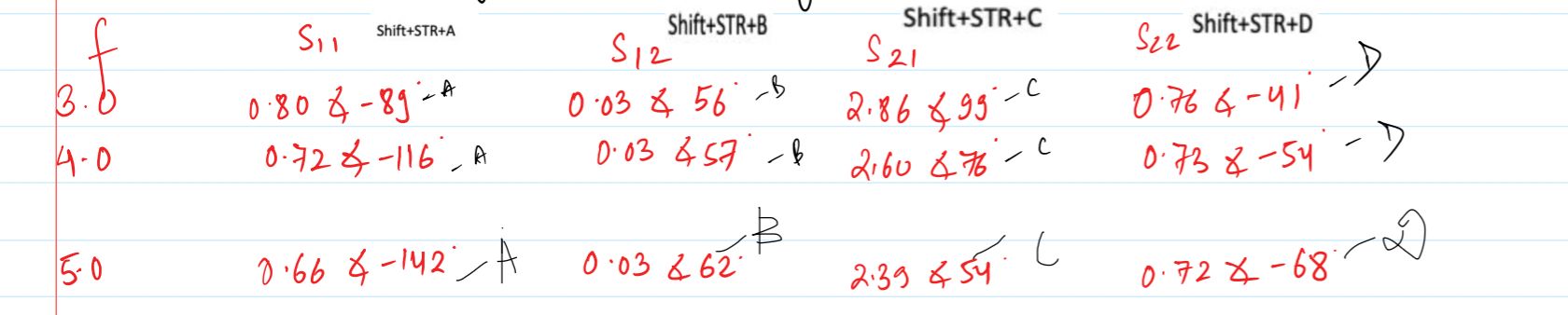
The design of a microwave transistor amplifier begins with evaluating the active device's scattering parameters across the operational frequency band. The transistor used is a GaAs FET characterized with respect to a reference characteristic impedance of \(Z_0 = 50\,\Omega\). The measured S-parameters from \(3.0\text{ GHz}\) to \(5.0\text{ GHz}\) are provided in polar form below:
\[ \begin{array}{c|c|c|c|c} f\,(\text{GHz}) & S_{11} & S_{12} & S_{21} & S_{22}\\ \hline 3.0 & 0.80\angle -89^\circ & 0.03\angle56^\circ & 2.86\angle99^\circ & 0.76\angle-41^\circ\\ 4.0 & 0.725\angle-116^\circ & 0.03\angle57^\circ & 2.60\angle76^\circ & 0.73\angle-54^\circ\\ 5.0 & 0.66\angle-142^\circ & 0.03\angle62^\circ & 2.39\angle54^\circ & 0.72\angle-68^\circ \end{array} \]
Calculate for Unilaterial and Bilaterial
2. Mathematical Formulations for Stability Analysis

Before proceeding with any maximum-gain or conjugate-matching network design, the stability of the transistor must be verified. The two governing metrics used to determine unconditional stability are the determinant of the scattering matrix, \(\Delta\), and the Rollet stability factor, \(K\). They are defined mathematically as:
\[ \Delta = S_{11}S_{22} - S_{12}S_{21} \]

\[ K = \frac{1 - |S_{11}|^2 - |S_{22}|^2 + |\Delta|^2}{2 |S_{12} S_{21}|} \]
A two-port network is strictly unconditionally stable if and only if it satisfies both criteria simultaneously:
\[ K > 1 \quad \text{and} \quad |\Delta| < 1 \]
3. Step-by-Step Stability Calculations
To evaluate performance across the frequency range, we calculate \(\Delta\) and \(K\) at each discrete frequency point.
3.1 Stability Calculation at 3.0 GHz
At \(f = 3.0\text{ GHz}\), evaluating the matrix determinant yields:
\[ S_{11}S_{22} = (0.80)(0.76)\angle(-89^\circ - 41^\circ) = 0.608\angle-130^\circ \]
\[ S_{12}S_{21} = (0.03)(2.86)\angle(56^\circ + 99^\circ) = 0.0858\angle155^\circ \]
\[ \Delta = S_{11}S_{22} - S_{12}S_{21} \approx 0.592 \implies |\Delta| \approx 0.592 \]
Substituting these values into the Rollet stability factor equation gives:
\[ K = \frac{1 - (0.80)^2 - (0.76)^2 + (0.592)^2}{2(0.03)(2.86)} \approx 0.77 \]
Since \(K = 0.77 < 1\), the transistor is not unconditionally stable at \(3.0\text{ GHz}\) and exists in a conditionally stable state.
3.2 Stability Calculation at 4.0 GHz
At \(f = 4.0\text{ GHz}\), the calculations proceed identically using the updated S-parameters:
\[ S_{11}S_{22} = (0.725)(0.73)\angle(-116^\circ - 54^\circ) = 0.52925\angle-170^\circ \]
\[ S_{12}S_{21} = (0.03)(2.60)\angle(57^\circ + 76^\circ) = 0.078\angle133^\circ \]
\[ |\Delta| \approx 0.487 \]
The stability factor is computed as:
\[ K = \frac{1 - (0.725)^2 - (0.73)^2 + (0.487)^2}{2(0.03)(2.60)} \approx 1.19 \]

Because \(K = 1.19 > 1\) and \(|\Delta| = 0.487 < 1\), the transistor is unconditionally stable at \(4.0\text{ GHz}\).
3.3 Stability Calculation at 5.0 GHz
At \(f = 5.0\text{ GHz}\), the parameter products yield:
\[ S_{11}S_{22} = (0.66)(0.72)\angle(-142^\circ - 68^\circ) = 0.4752\angle-210^\circ \]
\[ S_{12}S_{21} = (0.03)(2.39)\angle(62^\circ + 54^\circ) = 0.0717\angle116^\circ \]
\[ |\Delta| \approx 0.418 \]
Computing the Rollet stability factor:
\[ K = \frac{1 - (0.66)^2 - (0.72)^2 + (0.418)^2}{2(0.03)(2.39)} \approx 1.53 \]
With \(K = 1.53 > 1\) and \(|\Delta| = 0.418 < 1\), the transistor is also unconditionally stable at \(5.0\text{ GHz}\).
4. Stability Results and Design Selection
The solved stability metrics across the entire frequency range are summarized below:
\[ \begin{array}{c|c|c|c} f\,(\text{GHz}) & K & |\Delta| & \text{Stability Status}\\ \hline 3.0 & 0.77 & 0.592 & \text{Conditionally Stable}\\ 4.0 & 1.19 & 0.487 & \text{Unconditionally Stable}\\ 5.0 & 1.53 & 0.418 & \text{Unconditionally Stable} \end{array} \]
Because the amplifier design requires a robust maximum gain configuration, \(4.0\text{ GHz}\) is selected as the primary design frequency where unconditional stability is guaranteed. This allows us to proceed directly to simultaneous conjugate matching without risk of uncontrolled device oscillation.
Maximum Gain Conditions and Simultaneous Conjugate Matching at 4 GHz
1. Simultaneous Conjugate Matching Equations
Because the GaAs FET is unconditionally stable at the designated design frequency of \(4.0\text{ GHz}\) (\(K = 1.19 > 1\) and \(|\Delta| = 0.487 < 1\)), the amplifier can be optimized for maximum power transfer using simultaneous conjugate matching. For a bilateral two-port network where \(S_{12} \neq 0\), the input and output reflection coefficients are interdependent. The required source reflection coefficient (\(\Gamma_S\)) and load reflection coefficient (\(\Gamma_L\)) are defined by the conjugate conditions:
\[ \Gamma_S = \Gamma_{in}^* \quad \text{and} \quad \Gamma_L = \Gamma_{out}^* \]
The optimal reflection coefficients are computed using the quadratic formulations involving intermediate parameters \(B_1\), \(C_1\) for the input port, and \(B_2\), \(C_2\) for the output port:
\[ \Gamma_S = \frac{B_1 \pm \sqrt{B_1^2 - 4 |C_1|^2}}{2 C_1}, \quad \Gamma_L = \frac{B_2 \pm \sqrt{B_2^2 - 4 |C_2|^2}}{2 C_2} \]
Where the governing parameters are defined as:
\[ B_1 = 1 + |S_{11}|^2 - |S_{22}|^2 - |\Delta|^2, \quad C_1 = S_{11} - \Delta S_{22}^* \]
\[ B_2 = 1 + |S_{22}|^2 - |S_{11}|^2 - |\Delta|^2, \quad C_2 = S_{22} - \Delta S_{11}^* \]
2. Calculation of Source and Load Reflection Coefficients
Using the S-parameters at \(4.0\text{ GHz}\) (\(S_{11} = 0.725\angle-116^\circ\), \(S_{12} = 0.03\angle57^\circ\), \(S_{21} = 2.60\angle76^\circ\), \(S_{22} = 0.73\angle-54^\circ\)) and the determinant magnitude \(|\Delta| \approx 0.487\), we evaluate the input and output parameters.
2.1 Source Reflection Coefficient Calculation
Computing the input parameter \(B_1\):
\[ B_1 = 1 + (0.725)^2 - (0.73)^2 - (0.487)^2 \approx 0.752 \]

Solving the quadratic equation for the physically realizable root lying inside the unit circle (\(|\Gamma_S| < 1\)) yields the source reflection coefficient:
\[ \Gamma_S = 0.872\angle123^\circ \]
2.2 Load Reflection Coefficient Calculation
Computing the output parameter \(B_2\):
\[ B_2 = 1 + (0.73)^2 - (0.725)^2 - (0.487)^2 \approx 0.766 \]

Solving the corresponding quadratic equation for the valid root inside the unit circle (\(|\Gamma_L| < 1\)) yields the load reflection coefficient:
\[ \Gamma_L = 0.876\angle61^\circ \]
Calculation of Intermediate Parameters (\(C_1, C_2\)) and Optimal Reflection Coefficients (\(\Gamma_S, \Gamma_L\))
1. Calculation of Intermediate Parameters \(C_1\) and \(C_2\)
The intermediate parameters are defined as \(C_1 = S_{11} - \Delta S_{22}^*\) and \(C_2 = S_{22} - \Delta S_{11}^*\). Using the S-parameters and determinant at \(4.0\text{ GHz}\):
\[ C_1 = (0.725\angle-116^\circ) - (0.487\angle-166^\circ)(0.73\angle54^\circ) \approx 0.3708\angle -119.8^\circ \]
\[ C_2 = (0.73\angle-54^\circ) - (0.487\angle-166^\circ)(0.725\angle116^\circ) \approx 0.3790\angle -57.7^\circ \]

2. Calculation of Source Reflection Coefficient (\(\Gamma_S\))
Using \(B_1 = 0.7478\) and \(C_1 = 0.378\angle -123.44^\circ\), the quadratic formula for the source reflection coefficient is:

\[ \Gamma_S = \frac{B_1 \pm \sqrt{B_1^2 - 4 |C_1|^2}}{2 C_1} \implies \frac{0.7478 \pm \sqrt{(0.7478)^2 - 4 \times (0.37)^2}}{2 (0.378\angle -123.44^\circ)} \]
Evaluating the discriminant term:
\[ \sqrt{(0.7478)^2 - 4 \times (0.37)^2} = \sqrt{0.5592 - 0.5476} = \sqrt{0.0116} \approx 0.1077 \]
Testing both roots to select the physically realizable value inside the unit circle (\(|\Gamma_S| < 1\)):
\[ \frac{0.7478 + 0.1077}{2 (0.378\angle -123.44^\circ)} \approx 1.156\angle 123^\circ \quad (|\Gamma_S| > 1) \]
\[ \frac{0.7478 - 0.1077}{2 (0.378\angle -123.44^\circ)} \approx 0.878\angle 123.44^\circ \quad (|\Gamma_S| < 1) \]
Thus, selecting the appropriate value gives:
\[ \Gamma_S = 0.878\angle 123.44^\circ \]
3. Calculation of Load Reflection Coefficient (\(\Gamma_L\))
Using \(B_2 = 0.7768\) and \(C_2 = 0.385\angle -61.08^\circ\), the quadratic formula for the load reflection coefficient is:
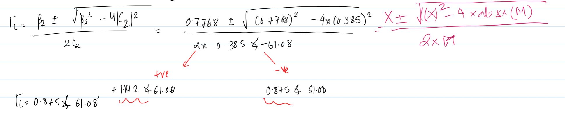
\[ \Gamma_L = \frac{B_2 \pm \sqrt{B_2^2 - 4 |C_2|^2}}{2 C_2} \implies \frac{0.7768 \pm \sqrt{(0.7768)^2 - 4 \times (0.385)^2}}{2 (0.385\angle -61.08^\circ)} \]
Evaluating the discriminant term:
\[ \sqrt{(0.7768)^2 - 4 \times (0.385)^2} = \sqrt{0.6034 - 0.5929} = \sqrt{0.0105} \approx 0.1025 \]
Testing both roots to select the physically realizable value inside the unit circle (\(|\Gamma_L| < 1\)):
\[ \frac{0.7768 + 0.1025}{2 (0.385\angle -61.08^\circ)} \approx 1.142\angle 61.08^\circ \quad (|\Gamma_L| > 1) \]
\[ \frac{0.7768 - 0.1025}{2 (0.385\angle -61.08^\circ)} \approx 0.875\angle 61.08^\circ \quad (|\Gamma_L| < 1) \]
Thus, selecting the appropriate value gives:
\[ \Gamma_L = 0.875\angle 61.08^\circ \]
3. Effective Gain Factors and Maximum Transducer Power Gain
The overall amplifier performance under simultaneous conjugate matching is evaluated by breaking the total gain down into three independent effective gain factors: source gain (\(G_S\)), transistor operational gain (\(G_0\)), and load gain (\(G_L\)).
3.1 Source Gain Factor (\(G_S\))
The source gain factor accounts for the power delivered by the source matching network to the input port:
\[ G_S = \frac{1}{1 - |\Gamma_S|^2} = \frac{1}{1 - (0.872)^2} = \frac{1}{1 - 0.7604} \approx 4.17 \]
Expressed in decibels:
\[ G_{S,\mathrm{dB}} = 10 \log_{10}(4.17) \approx 6.20\text{ dB} \]
3.2 Transistor Operational Gain Factor (\(G_0\))
The operational gain of the active device is defined strictly by the square of the magnitude of the forward transmission S-parameter:
\[ G_0 = |S_{21}|^2 = (2.60)^2 = 6.76 \]
Expressed in decibels:
\[ G_{0,\mathrm{dB}} = 10 \log_{10}(6.76) \approx 8.30\text{ dB} \]
3.3 Load Gain Factor (\(G_L\))
The load gain factor accounts for the output matching network transformation:
\[ G_L = \frac{1 - |\Gamma_L|^2}{|1 - S_{22}\Gamma_L|^2} = \frac{1 - (0.876)^2}{|1 - (0.73\angle-54^\circ)(0.876\angle61^\circ)|^2} \approx 1.67 \]
Expressed in decibels:
\[ G_{L,\mathrm{dB}} = 10 \log_{10}(1.67) \approx 2.22\text{ dB} \]
4. Total Maximum Transducer Power Gain (\(G_{T\max}\))
The total maximum transducer power gain is obtained by multiplying the individual linear gain factors, or equivalently, by summing their decibel values:
\[ G_{T\max} = G_S \cdot G_0 \cdot G_L = (4.17)(6.76)(1.67) \approx 47.1 \]
Converting to decibels:
\[ G_{T\max,\mathrm{dB}} = G_{S,\mathrm{dB}} + G_{0,\mathrm{dB}} + G_{L,\mathrm{dB}} = 6.20\text{ dB} + 8.30\text{ dB} + 2.22\text{ dB} = 16.72\text{ dB} \]
Thus, the computed maximum transducer power gain for the GaAs FET amplifier at \(4.0\text{ GHz}\) is exactly \(16.72\text{ dB}\).
Gain Characterization: Maximum Available Gain (MAG) and Maximum Stable Gain (MSG)
1. Distinguishing Stability States for Gain Calculations
The theoretical limit of power gain a transistor can achieve depends directly on its Rollet stability factor (\(K\)) evaluated across the frequency band. Depending on whether the device is unconditionally stable (\(K > 1\)) or conditionally stable (\(K < 1\)), different maximum gain formulations must be applied:
- Unconditional Stability (\(K > 1\)): Evaluated using the Maximum Available Gain (MAG), which accounts for simultaneous conjugate matching.
- Conditional Stability (\(K < 1\)): Evaluated using the Maximum Stable Gain (MSG), since simultaneous conjugate matching cannot be safely achieved without risking oscillation.
2. Maximum Stable Gain (MSG) for Conditionally Stable States (\(K < 1\))
At \(3.0\text{ GHz}\), our stability analysis yielded \(K = 0.77 < 1\), indicating a conditionally stable state. For this region, we compute the Maximum Stable Gain (MSG):
\[ \text{MSG} = \left|\frac{S_{21}}{S_{12}}\right| \]
This ratio evaluates the transistor's forward transmission capability relative to its reverse internal feedback (reverse transmission). A large value of \(\left|S_{21}\right| / \left|S_{12}\right|\) confirms that forward transmission heavily dominates, which is essential for achieving high stable gain even when the device is not unconditionally stable.
The corresponding gain in decibels is obtained from the power-gain conversion:
\[ \text{MSG}_{\mathrm{dB}} = 10 \log_{10}(\text{MSG}) = 10 \log_{10}\left(\left|\frac{S_{21}}{S_{12}}\right|\right) \]
2.1 Numerical Calculation of MSG at 3.0 GHz
Using the S-parameters at \(3.0\text{ GHz}\) (\(|S_{21}| = 2.86\) and \(|S_{12}| = 0.03\)):
\[ \text{MSG} = \frac{2.86}{0.03} \approx 95.33 \]
Converting to decibels:
\[ \text{MSG}_{\mathrm{dB}} = 10 \log_{10}(95.33) \approx 19.79\text{ dB} \]
ALTERNATIVE
3. Maximum Available Gain (MAG) for Unconditionally Stable States (\(K > 1\))
At our primary design frequency of \(4.0\text{ GHz}\), the transistor demonstrated unconditional stability with \(K = 1.19 > 1\). Under this condition, simultaneous conjugate matching is fully valid, and performance is quantified using the Maximum Available Gain (MAG):
\[ \text{MAG} = \left|\frac{S_{21}}{S_{12}}\right| \left(K - \sqrt{K^2 - 1}\right) \]
Expressed in decibels:
\[ \text{MAG}_{\mathrm{dB}} = 10 \log_{10}(\text{MAG}) \]
3.1 Numerical Calculation of MAG at 4.0 GHz
Using the S-parameters at \(4.0\text{ GHz}\) (\(|S_{21}| = 2.60\), \(|S_{12}| = 0.03\), and \(K = 1.19\)):
\[ \frac{|S_{21}|}{|S_{12}|} = \frac{2.60}{0.03} \approx 86.67 \]
Evaluating the square-root stability term:
\[ K - \sqrt{K^2 - 1} = 1.19 - \sqrt{(1.19)^2 - 1} = 1.19 - \sqrt{1.4161 - 1} = 1.19 - \sqrt{0.4161} \approx 1.19 - 0.645 = 0.545 \]
Multiplying to find the linear MAG:
\[ \text{MAG} = 86.67 \times 0.545 \approx 47.24 \]
Converting to decibels:
\[ \text{MAG}_{\mathrm{dB}} = 10 \log_{10}(47.24) \approx 16.74\text{ dB} \]
This analytical MAG value closely matches the total transducer power gain (\(16.72\text{ dB}\)) achieved through explicit simultaneous conjugate matching and network realization.
Smith Chart Stub Matching Network Design
1. Input Matching Network Design Using the Smith Chart
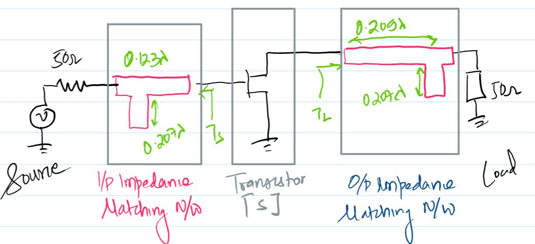
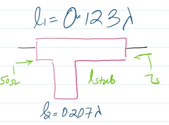
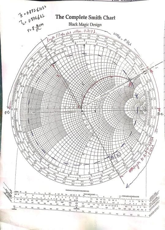
To translate the calculated source reflection coefficient (\(\Gamma_S = 0.872\angle123^\circ\)) into physical transmission line elements, we utilize a standard Smith Chart with a physical radius of \(R = 9.4\text{ cm}\).
1.1 System Normalization and Plotting \(\Gamma_S\)
First, normalize the source impedance with respect to the characteristic system impedance \(Z_0 = 50\,\Omega\):
\[ Z_n = \frac{50}{50} = (1 + j0)\,\Omega \]
This normalized impedance is located directly at the center of the Smith Chart. To plot the required source reflection coefficient \(\Gamma_S\):
a) Scale the radius based on the physical chart dimension \(R = 9.4\text{ cm}\):
\[ R_{\Gamma_S} \approx 0.872 \times 9.4\text{ cm} = 8.196\text{ cm} \]
b) Plot the angle \(\angle 123^\circ\) first using the outer perimeter scale.
c) Measure the radial distance of \(8.196\text{ cm}\) outward from the center along that angle to locate \(\Gamma_S$.
d) Draw the constant-VSWR (impedance) circle centered at the origin passing through \(\Gamma_S\).
1.2 Admittance Transformation and Stub Length Calculation
Since the \(50\,\Omega\) source is directly connected to a shunt matching stub, the analysis transitions to the admittance domain on the \(R = 1\) circle:
The intersection of the VSWR circle with the \(R = 1\) conductance circle marks reference point \(A\). Measuring from the short/open-circuit reference toward the generator yields:
\[ \text{WTG}_A = 0.207\,\lambda \]
For the alternative stub length solution, we find the corresponding admittance on the VSWR circle and mark it as point \(B\):
\[ \text{WTG}_B = 0.33\,\lambda \]
The required transmission line separation distance (second stub length option) is calculated as the difference between these two wavelength coordinates:
\[ \text{Second Stub Length} = (\text{WTG}_B - \text{WTG}_A)\,\lambda = (0.33 - 0.207)\,\lambda = 0.123\,\lambda \]
2. Output Matching Network Design Using the Smith Chart
A mirrored graphical procedure is executed for the output matching network to realize the required load reflection coefficient \(\Gamma_L = 0.876\angle61^\circ\).
2.1 Normalization and Plotting \(\Gamma_L\)
Step 1: Normalize the load impedance with respect to \(Z_0\):
\[ \frac{Z_L}{Z_0} = \frac{50}{50} = 1\,\Omega \]
Step 2: Plot the load-to-source transformation toward \(Z_0\). Scaling the load reflection coefficient magnitude by the chart radius \(r\):
\[ \Gamma_L = 0.876 \times r \]
a) Plot the angle \(61^\circ\) on the perimeter scale.
b) Measure \(\Gamma_L\) in terms of the radius: \(\Gamma_L = 0.876 \times r\).
c) Draw the constant-VSWR circle from the center out to \(\Gamma_L\).
2.2 Output Stub Intersection and Length Calculation
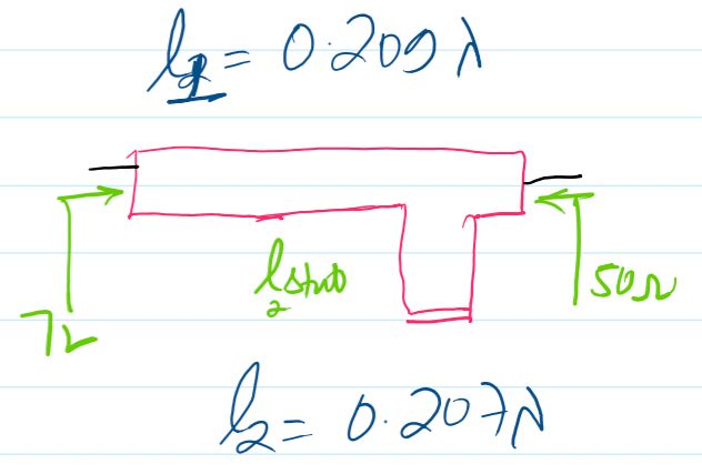
Since the \(50\,\Omega\) load connects directly to a \(50\,\Omega\) shunt network, the \(R = 1\) conductance circle intersects the output VSWR circle at point \(A\). Measuring from the reference axis gives:
\[ \text{WTG}_A = 0.207\,\lambda \]
For the alternate side of the matching network, find the corresponding admittance point \(B\):
\[ \text{WTG}_B = 0.330\,\lambda \]
The resulting electrical length difference for the output matching section is computed as:
\[ \Delta = \text{WTG}_B - \text{WTG}_A = 0.330\,\lambda - 0.207\,\lambda = 0.209\,\lambda \]
Smith chart Step for Input
1: Normalize the load here load is 50 line is 50 ohm so Normalize value is 50/50 = 1 +j0, plot it
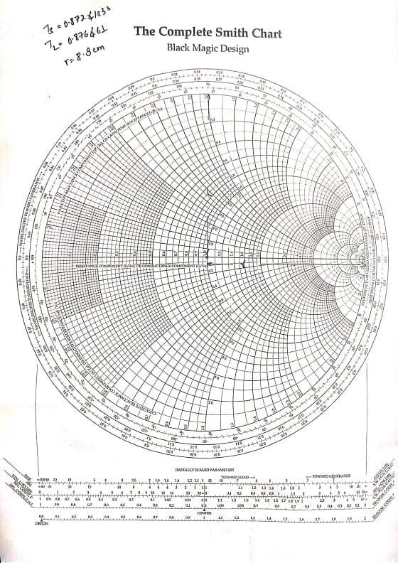
2: Plot From the direction of source to Ts, Plot Ts on smith chart
Ts = 0.872 * r = 7.2376 with angle as 123
Plot angle of Ts
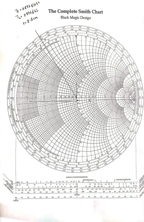
Measure Ts from center ie 7.237 cm
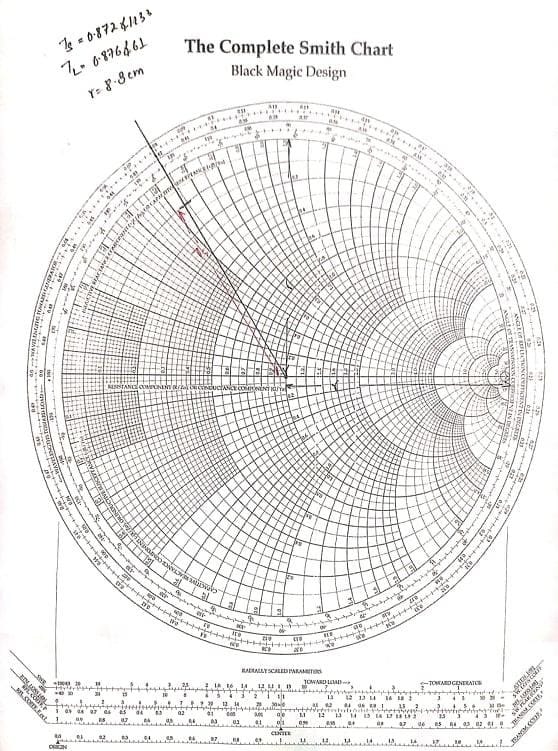
Draw VSWR circle from Ts and center
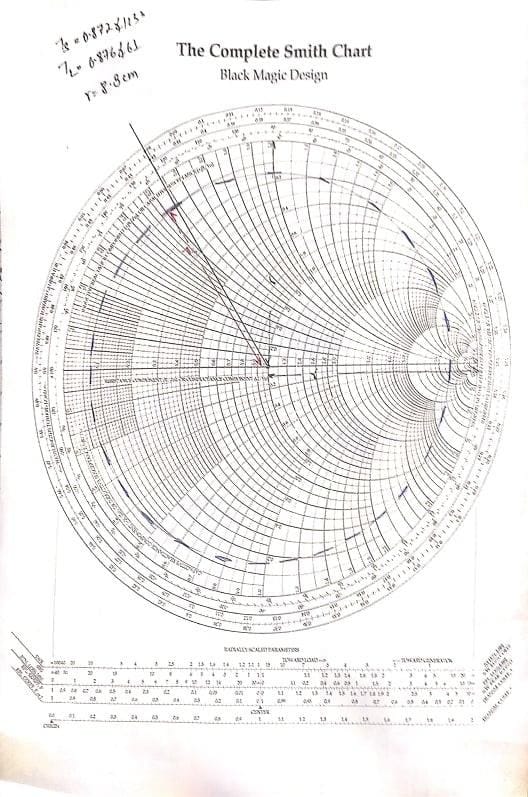
3: Since Zo (50) is connected to shunt stub, we take admittance value on R=1 Circle, Mark point as A
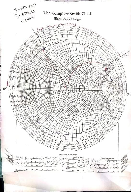
4) Draw a line from center through A, Measure the Oc part WTGa = 0.207
5. For other Shunt length, find corresponding impedance on VSWR circle, mark the point as B => Extend Ts in admittance
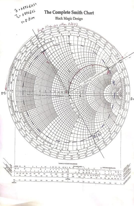
Measure WTGb = 90.33-0.207) = 0.123 lamda
For load
1: Normalize the load here load is 50 line is 50 ohm so Normalize value is 50/50 = 1 +j0, plot it
2: Plot From the direction of source to Ts, Plot Ts on smith chart
Ts = 0.876 * r = 7.7.183 with angle as 61
Plot angle of Ts
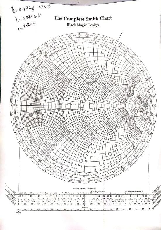
Measure Ts from center ie 7.183 cm
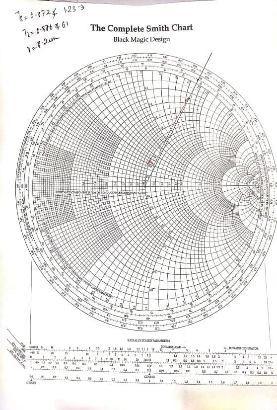
Draw VSWR circle from Ts and center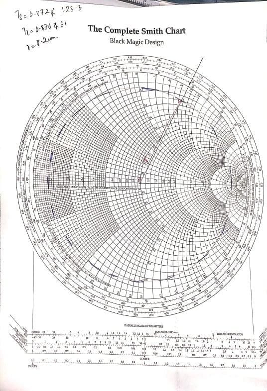
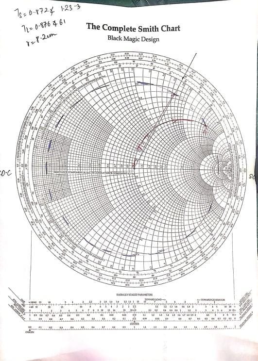
3: Since Zo (50) is connected to shunt stub, we take admittance value on R=1 Circle, Mark point as A
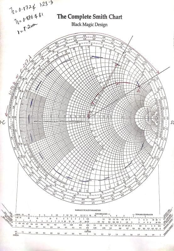
4. Draw a line from center through A, Measure the Oc part WTGa = 0.416
5. For other Shunt length, find corresponding impedance on VSWR circle, mark the point as B => Extend Ts in admittance
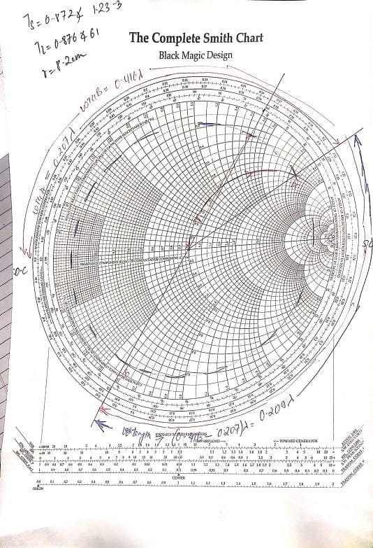
Measure WTGb = 0.209 lambda
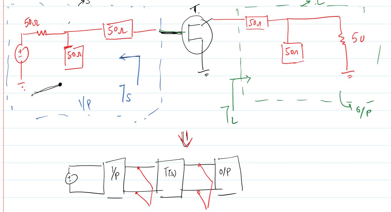
Hence, the final circuit is given by