Microwave Amplifier Design
Microwave Amplifier Design and Two-Port Power Gains
1. Introduction to Microwave Amplifier Design
Microwave amplifier design is concerned with developing amplifying circuits that can increase the power or voltage level of high-frequency signals while maintaining the required gain, stability, bandwidth, noise performance, and power-handling capability. At microwave frequencies, amplifier design is more complicated than conventional low-frequency amplifier design because parasitic effects, transmission-line behavior, impedance matching, and device limitations become increasingly important. In the early development of microwave engineering, amplification was mainly achieved using vacuum-tube devices such as klystrons and travelling-wave tubes (TWTs). Solid-state reflection amplifiers were also developed using the negative-resistance characteristics of devices such as tunnel diodes and varactor diodes. Although these devices played an important role in the development of microwave technology, the introduction and continuous improvement of semiconductor transistor devices made compact and reliable microwave amplifiers much more practical. Modern RF and microwave amplifiers are therefore largely based on transistor technologies such as silicon bipolar junction transistors (Si BJTs), gallium arsenide (GaAs) devices, silicon-germanium (SiGe) devices, indium phosphide (InP) FETs, and gallium arsenide high-electron-mobility transistors (GaAs HEMTs). These devices can operate at frequencies well above 100 GHz and can be designed for applications requiring small physical size, low noise figure, wide bandwidth, and medium to high output power. Because of these requirements, microwave amplifier design is not simply a matter of selecting a transistor and applying a bias voltage. The designer must understand how the device behaves as a two-port network and must determine whether the required gain can be achieved while maintaining stable operation and acceptable input and output matching.
1.1 Development of Microwave Amplifiers
The development of microwave amplifiers has followed the evolution of high-frequency electronic devices. Early microwave systems depended heavily on vacuum-tube technology because conventional low-frequency transistor circuits could not provide sufficient performance at microwave frequencies. Klystrons provided high-power amplification by using the interaction between an electron beam and resonant cavities, while travelling-wave tubes used a continuous interaction between an electron beam and a travelling electromagnetic wave to provide wideband amplification. Another approach was the use of solid-state reflection amplifiers, in which the negative-resistance characteristics of devices such as tunnel diodes and varactor diodes were used to produce amplification. These approaches established many of the fundamental principles used in microwave amplification, but the physical size, operating requirements, bandwidth limitations, and practical implementation of such devices encouraged the development of semiconductor microwave technology. Transistor devices gradually became the preferred choice for a large range of RF and microwave applications because they offered smaller size, lower operating requirements, easier integration, and improved reliability. Modern semiconductor technologies have extended transistor operation into very high-frequency regions, making transistor amplifiers suitable for communication systems, radar, instrumentation, satellite systems, wireless systems, and many other microwave applications.
1.1.1 Modern Transistor Microwave Amplifiers
Modern microwave amplifiers can be implemented using several semiconductor technologies, with the choice depending on the required frequency range, gain, noise performance, output power, and operating environment. Silicon BJTs are useful in many RF applications, while GaAs-based devices provide favorable high-frequency characteristics because of the properties of the semiconductor material. SiGe technology is particularly useful where high-frequency performance must be combined with the advantages of silicon-based manufacturing. InP FETs and GaAs HEMTs are widely associated with very high-frequency operation because their device structures provide excellent electron transport characteristics. The high electron mobility of a HEMT allows it to operate effectively at very high frequencies, making such devices important in low-noise and high-frequency microwave circuits. Transistor amplifiers can operate at frequencies exceeding 100 GHz, although the practical operating frequency depends strongly on the particular device technology and circuit design. At these frequencies, the amplifier must be designed as a microwave network rather than treated as a simple lumped-element circuit. Transmission-line effects, device parasitics, reflection coefficients, and impedance matching all influence the final amplifier performance.
1.2 Important Considerations in Microwave Amplifier Design
Several parameters must be considered when designing a transistor-based microwave amplifier. One of the most important tools is the use of S-parameters, which describe the relationship between incident and reflected travelling waves at the ports of a microwave network. S-parameters are particularly convenient at high frequencies because direct measurement of voltages and currents at the device terminals becomes difficult, whereas incident and reflected waves can be measured using microwave test equipment. Along with S-parameters, stability is a fundamental consideration because an amplifier must amplify the desired signal without becoming unstable or developing unwanted oscillations. The designer must also determine the maximum gain that the device can provide under the specified operating conditions and, when a particular gain rather than the absolute maximum gain is required, select an appropriate operating point and matching network to obtain the specified gain. Noise figure is another critical parameter, especially in receiver systems where a small amount of additional noise can significantly affect the sensitivity of the complete system. Therefore, practical microwave amplifier design involves balancing gain, stability, noise figure, bandwidth, and power-handling capability rather than optimizing only one parameter.
2. Two-Port Power Gains of a Microwave Amplifier
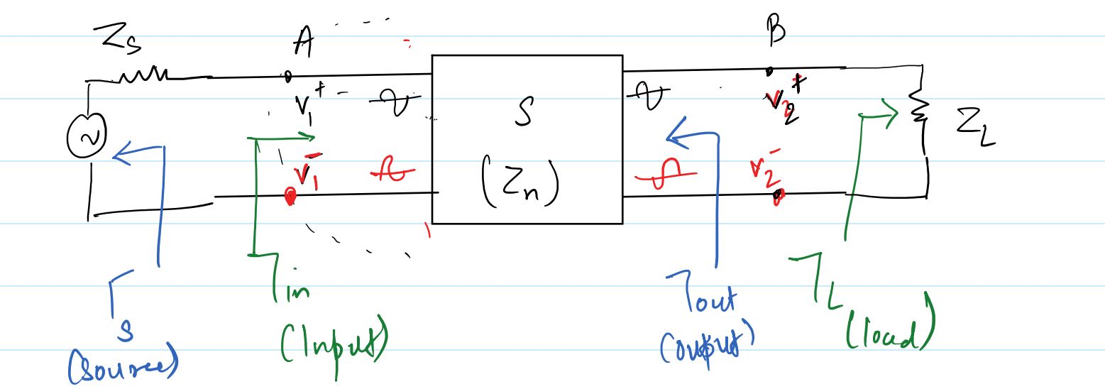
A transistor microwave amplifier can be represented as a two-port network with a source connected to its input port and a load connected to its output port. Different definitions of power gain are used because the actual gain of the amplifier depends not only on the characteristics of the two-port network but also on how the source and load are connected to it. Three important quantities are the operating power gain, the available power gain, and the transducer power gain. The operating power gain, denoted by \(G_P\), compares the power delivered to the load with the power delivered to the input of the two-port network. The available power gain, denoted by \(G_A\), compares the maximum power available from the two-port network with the maximum power available from the source. The transducer power gain, denoted by \(G_T\), compares the power actually delivered to the load with the maximum power available from the source. These definitions are important because they describe different aspects of amplifier performance and have different dependencies on the source and load impedances.
2.1 Operating Power Gain
The operating power gain is defined as the ratio of the power delivered to the load \(P_L\) to the power delivered to the input of the two-port network \(P_{in}\). It is therefore written as
\[ G_P=\frac{P_L}{P_{in}} \]
The operating power gain describes how much the two-port network increases the power that it receives at its input before delivering power to the load. An important characteristic of this gain is that, in its basic definition, it is independent of the source impedance \(Z_S\), although the characteristics of some active microwave devices may themselves depend on the source impedance. The load impedance \(Z_L\), however, directly affects the amount of power that can be delivered by the amplifier. This is why the operating gain becomes particularly useful when analyzing the performance of an amplifier after the input power delivered to the active device has already been established.
2.2 Available Power Gain
The available power gain is defined using the maximum power that can be obtained from both the source and the two-port network. It is expressed as the ratio of the power available from the network \(P_{avn}\) to the power available from the source \(P_{ars}\).
\[ G_A=\frac{P_{avn}}{P_{ars}} \]
The available power gain assumes conjugate matching at both the source and load conditions so that the maximum available power can be transferred. Unlike the operating power gain, the available power gain depends on the source impedance \(Z_S\), because the available power from the source depends on the source matching condition. Under its standard definition, however, it does not depend directly on the external load impedance \(Z_L\), because the output of the two-port network is considered under the condition that the load is conjugately matched to obtain the maximum available output power. This makes \(G_A\) useful for evaluating the inherent power-delivery capability of the amplifier network when maximum power transfer conditions are considered.
2.3 Transducer Power Gain
The transducer power gain provides a direct measure of the overall power-transfer performance of the amplifier from the source to the load. It is defined as the ratio of the power actually delivered to the load \(P_L\) to the power available from the source \(P_{ars}\).
\[ G_T=\frac{P_L}{P_{ars}} \]
Unlike the operating power gain and available power gain, the transducer power gain depends on both the source impedance \(Z_S\) and the load impedance \(Z_L\). This occurs because the actual power delivered to the load depends on the output matching condition, while the power available from the source depends on the input matching condition. Consequently, \(G_T\) is particularly important in practical microwave amplifier design because it considers the complete source-to-amplifier-to-load power-transfer path rather than considering only the internal gain of the two-port network.
2.4 Reflection Coefficients at the Source and Load
The source and load matching conditions can be described conveniently using reflection coefficients. The reflection coefficient looking toward the load is denoted by \(\Gamma_L\), while the reflection coefficient looking toward the source is denoted by \(\Gamma_S\). With a reference impedance \(Z_0\), these reflection coefficients are defined in terms of the corresponding impedances as
\[ \Gamma_L=\frac{Z_L-Z_0}{Z_L+Z_0} \]
\[ \Gamma_S=\frac{Z_S-Z_0}{Z_S+Z_0} \]
These coefficients indicate the degree of impedance mismatch between the two-port network and the external source or load. When the source or load is perfectly matched to the reference impedance, its corresponding reflection coefficient becomes zero. Thus, \(\Gamma_S=0\) represents a matched source and \(\Gamma_L=0\) represents a matched load. In microwave amplifier analysis, reflection coefficients are generally more convenient than directly working with impedances because S-parameters and travelling-wave quantities are naturally expressed in terms of incident and reflected waves. The three power gains can therefore be related to the source and load reflection coefficients as the amplifier analysis progresses.
2.5 Conjugate Matching and Maximum Power Gain
For maximum power transfer, the input and output of the two-port network must satisfy the appropriate conjugate-matching conditions. When the input and output are both conjugately matched to the two-port network, the power delivered from the source to the amplifier and from the amplifier to the load is maximized. Under this condition, the three power-gain definitions become equal, giving
\[ G_P=G_A=G_T \]
This equality is an important result in microwave amplifier design because it shows that the operating, available, and transducer power gains can have the same value when the appropriate maximum-power-transfer conditions are satisfied. In a practical amplifier, however, perfect conjugate matching may not always be selected because the designer may need to prioritize other requirements such as stability, bandwidth, noise figure, or a specified gain. Therefore, the gain definitions must be understood individually before selecting the source and load matching conditions. The relationships among \(G_P\), \(G_A\), and \(G_T\), together with the reflection coefficients and S-parameters of the two-port network, form the foundation for the detailed gain analysis of microwave amplifiers.
3. S-Parameter Analysis of Input and Output Reflection Coefficients
The input and output reflection coefficients are fundamental quantities in microwave amplifier design because they describe how the amplifier interacts with the source and load connected to its two ports. For a two-port microwave network, the relationship between the incident and reflected waves is conveniently represented using S-parameters. Let \(V_1^+\) and \(V_2^+\) represent the incident waves at ports 1 and 2, while \(V_1^-\) and \(V_2^-\) represent the reflected waves from those ports. The S-parameter equations for the two-port network can therefore be written as
\[ V_1^- = S_{11}V_1^+ + S_{12}V_2^+ \]
\[ V_2^- = S_{21}V_1^+ + S_{22}V_2^+ \]
Here, \(S_{11}\) represents the input reflection coefficient when port 2 is terminated in the reference impedance, \(S_{22}\) represents the output reflection coefficient when port 1 is terminated in the reference impedance, \(S_{21}\) represents the forward transmission coefficient, and \(S_{12}\) represents the reverse transmission coefficient. When the amplifier is connected to an actual source and load, the waves returning from the load and source are fed back into the two-port network. Consequently, the effective input and output reflection coefficients are not determined by \(S_{11}\) and \(S_{22}\) alone. They also depend on the opposite-port reflection coefficients and the forward and reverse transmission characteristics of the device.
3.1 Input Reflection Coefficient
Consider first the input side of the two-port amplifier. The load connected to port 2 produces a reflected wave that returns toward the two-port network. The load reflection coefficient is defined as the ratio of the reflected wave to the incident wave at the load, so that
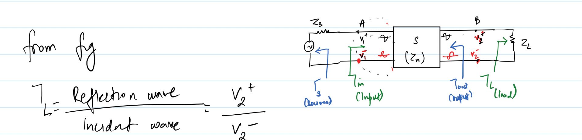
\[ \Gamma_L=\frac{V_2^+}{V_2^-} \]
or, equivalently,
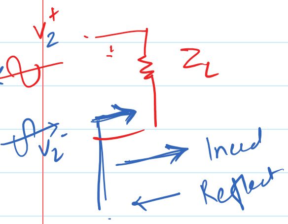
\[ V_2^+=\Gamma_LV_2^- \]
The first S-parameter equation is
\[ V_1^+=S_{11}V_1^+ + S_{12}V_2^+ \]
To avoid ambiguity between incident and reflected waves, the correct two-port wave relation at port 1 is written as
\[ V_1^-=S_{11}V_1^+ + S_{12}V_2^+ \]
Substituting \(V_2^+=\Gamma_LV_2^-\) gives
\[ V_1^-=S_{11}V_1^+ + S_{12}\Gamma_LV_2^- \]
The second S-parameter equation is
\[ V_2^-=S_{21}V_1^+ + S_{22}V_2^+ \]
Using the load relationship \(V_2^+=\Gamma_LV_2^-\), this becomes
\[ V_2^-=S_{21}V_1^+ + S_{22}\Gamma_LV_2^- \]
Collecting the terms containing \(V_2^-\) on the left side gives
\[ V_2^-(1-S_{22}\Gamma_L)=S_{21}V_1^+ \]
Therefore, the wave travelling toward the load can be expressed in terms of the incident wave at port 1 as
\[ V_2^-=\frac{S_{21}}{1-S_{22}\Gamma_L}V_1^+ \]
Substituting this result into the expression for \(V_1^-\) gives
\[ V_1^-=S_{11}V_1^+ + S_{12}\Gamma_L\left(\frac{S_{21}}{1-S_{22}\Gamma_L}V_1^+\right) \]
Taking \(V_1^+\) as a common factor, we obtain
\[ V_1^-= \left[ S_{11}+ \frac{S_{12}S_{21}\Gamma_L} {1-S_{22}\Gamma_L} \right]V_1^+ \]
The input reflection coefficient is defined as the ratio of the reflected wave at port 1 to the incident wave at port 1. Hence,
\[ \Gamma_{in}=\frac{V_1^-}{V_1^+} \]
Substituting the previous result gives the effective input reflection coefficient of the loaded two-port network as
\[ \boxed{ \Gamma_{in} = S_{11} + \frac{S_{12}S_{21}\Gamma_L} {1-S_{22}\Gamma_L} } \]
This expression shows that the input reflection coefficient depends on more than the input S-parameter \(S_{11}\). The load reflection coefficient \(\Gamma_L\) influences the input behavior through the reverse transmission parameter \(S_{12}\) and the forward transmission parameter \(S_{21}\). The term involving \(S_{12}S_{21}\Gamma_L\) represents the effect of the signal travelling through the amplifier toward the load, being reflected by the load, and then coupling back toward the input. Therefore, a change in the load impedance can change the effective input impedance and input reflection coefficient of an active microwave device.
3.2 Input Reflection Coefficient in Terms of Input Impedance
The input reflection coefficient can also be expressed in terms of the input impedance seen by the source. If the characteristic or reference impedance of the system is \(Z_0\), the relationship between the input reflection coefficient and input impedance is
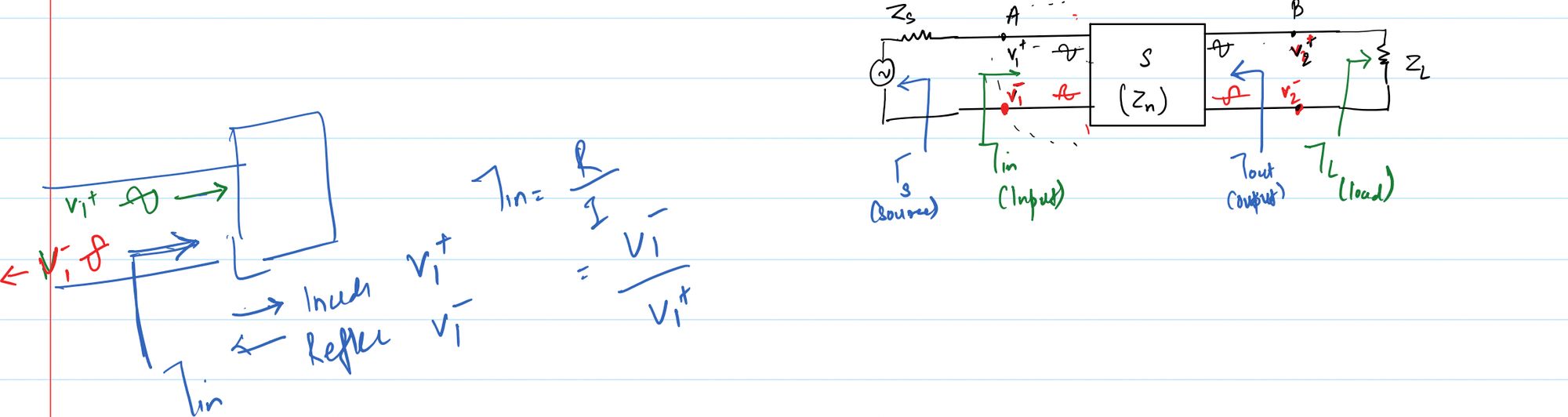
\[ \Gamma_{in}=\frac{Z_{in}-Z_0}{Z_{in}+Z_0} \]
Combining this relationship with the S-parameter result gives
\[ \boxed{ \Gamma_{in} = S_{11} + \frac{S_{12}S_{21}\Gamma_L} {1-S_{22}\Gamma_L} = \frac{Z_{in}-Z_0}{Z_{in}+Z_0} } \]
Thus, once the S-parameters of the amplifier and the load reflection coefficient are known, the effective input reflection coefficient can be determined and, if required, converted into the corresponding input impedance. This relationship is especially important in matching-network design because it allows the designer to determine how the chosen load affects the impedance presented to the source.
3.3 Output Reflection Coefficient
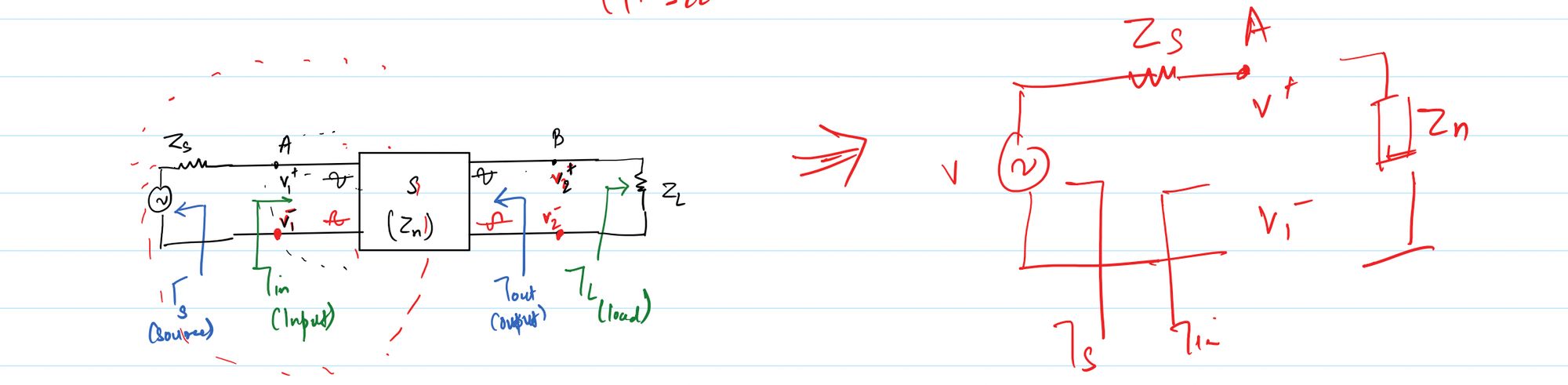
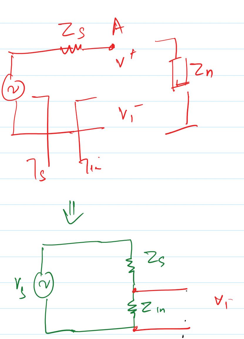
A similar procedure can be used to determine the effective output reflection coefficient of the two-port amplifier. In this case, the source connected to port 1 produces a reflected wave that returns toward the source. The source reflection coefficient can be expressed as
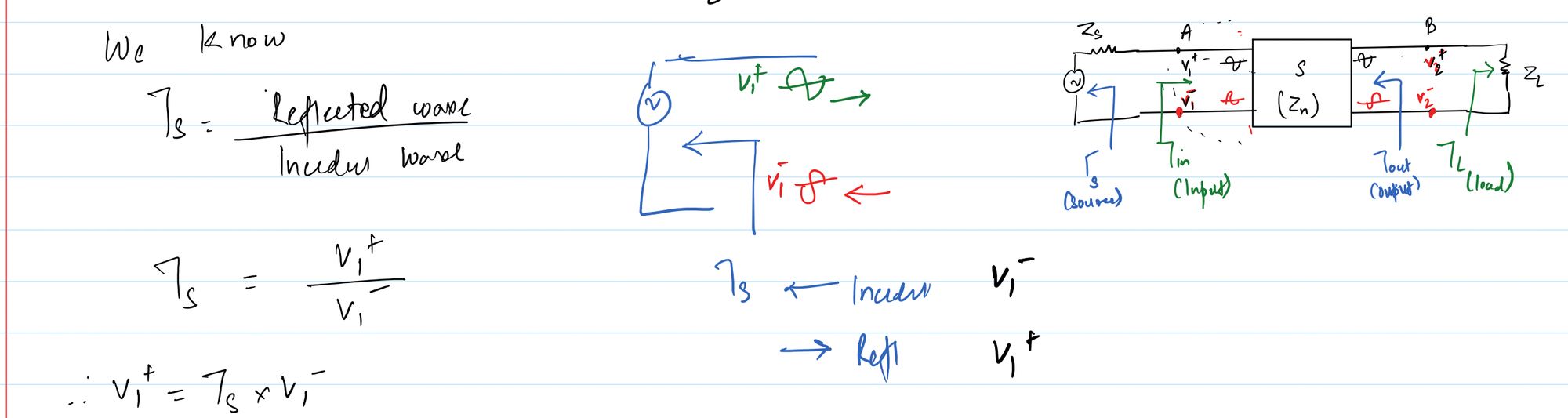
\[ \Gamma_S=\frac{V_1^+}{V_1^-} \]
or
\[ V_1^+=\Gamma_SV_1^- \]
Starting with the first S-parameter equation,
\[ V_1^-=S_{11}V_1^+ + S_{12}V_2^+ \]
and substituting \(V_1^+=\Gamma_SV_1^-\), we obtain
\[ V_1^-=S_{11}\Gamma_SV_1^- + S_{12}V_2^+ \]
Rearranging the terms gives
\[ V_1^-(1-S_{11}\Gamma_S)=S_{12}V_2^+ \]
Therefore,
\[ V_1^-= \frac{S_{12}} {1-S_{11}\Gamma_S}V_2^+ \]
Now consider the second S-parameter equation,
\[ V_2^-=S_{21}V_1^+ + S_{22}V_2^+ \]
Substituting \(V_1^+=\Gamma_SV_1^-\) gives
\[ V_2^-=S_{21}\Gamma_SV_1^- + S_{22}V_2^+ \]
Using the previously obtained expression for \(V_1^-\), we get
\[ V_2^-= S_{21}\Gamma_S \left( \frac{S_{12}} {1-S_{11}\Gamma_S} \right)V_2^+ + S_{22}V_2^+ \]
Dividing both sides by \(V_2^+\) gives
\[ \frac{V_2^-}{V_2^+} = S_{22} + \frac{S_{12}S_{21}\Gamma_S} {1-S_{11}\Gamma_S} \]
The effective output reflection coefficient is defined as the ratio of the reflected wave at port 2 to the incident wave at port 2. Hence,
\[ \Gamma_{out}=\frac{V_2^-}{V_2^+} \]
Therefore, the output reflection coefficient of the two-port network when the source is connected to the input port is
\[ \boxed{ \Gamma_{out} = S_{22} + \frac{S_{12}S_{21}\Gamma_S} {1-S_{11}\Gamma_S} } \]
The expression for \(\Gamma_{out}\) has a form similar to the expression for \(\Gamma_{in}\), but the roles of the source and load are interchanged. The output reflection coefficient is therefore affected by the source reflection coefficient \(\Gamma_S\), as well as by the S-parameters of the active device. This result is important because changing the source impedance can alter the impedance presented at the output of a microwave amplifier. In an active two-port network, the input and output ports are therefore generally coupled through the forward and reverse transmission parameters, and the source and load cannot always be treated as completely independent.
3.4 Importance of the Reflection Coefficient Relationships
The expressions for \(\Gamma_{in}\) and \(\Gamma_{out}\) provide the foundation for the subsequent analysis of microwave amplifier gain and matching. They show how the source and load terminations interact with the internal S-parameters of the amplifier and determine the actual input and output behavior of the complete two-port network. These relationships are also essential when deriving the operating power gain, available power gain, and transducer power gain because each gain depends on the amount of power entering the amplifier, the amount of power transferred through the device, and the amount of power ultimately delivered to the load. In particular, the terms \(1-S_{22}\Gamma_L\) and \(1-S_{11}\Gamma_S\) represent the effects of multiple reflections between the amplifier and its terminations. Understanding these relationships makes it possible to move from basic S-parameter analysis to a complete mathematical description of amplifier power gain and matching conditions.
4. Derivation of Power Gain, Available Gain and Transducer Gain
The power-gain analysis of a microwave amplifier becomes clearer once the source and load are represented by their reflection coefficients and the amplifier itself is described by its S-parameters. The three important gain quantities are the operating power gain \(G_P\), available power gain \(G_A\), and transducer power gain \(G_T\). Although these gains are related, each one uses a different reference power and therefore describes a different aspect of amplifier performance. The operating power gain compares the power delivered to the load with the power delivered to the input of the two-port network, the available power gain compares the maximum power available from the network with the maximum power available from the source, and the transducer power gain compares the actual power delivered to the load with the power available from the source. The derivations below use the travelling-wave representation of the two-port network and the reflection coefficients developed in the previous section.
4.1 Power Gain of a Two-Port Amplifier
For a two-port network, the power delivered to the load is determined by the difference between the power carried by the wave travelling toward the load and the power carried by the wave reflected from the load. Using normalized travelling-wave quantities, the load power can be written in terms of \(b_2\) and \(a_2\) as
\[ P_L=\frac{1}{2}\left(|b_2|^2-|a_2|^2\right) \]
Since the load reflection coefficient is defined by \(a_2=\Gamma_Lb_2\), the load power becomes
\[ P_L=\frac{1}{2}|b_2|^2\left(1-|\Gamma_L|^2\right) \]
From the two-port S-parameter relationship, the output wave can be written as
\[ b_2=S_{21}a_1+S_{22}a_2 \]
Using \(a_2=\Gamma_Lb_2\), this relation becomes
\[ b_2=S_{21}a_1+S_{22}\Gamma_Lb_2 \]
Rearranging gives
\[ b_2(1-S_{22}\Gamma_L)=S_{21}a_1 \]
and therefore
\[ b_2=\frac{S_{21}}{1-S_{22}\Gamma_L}a_1 \]
Substituting this expression into the load-power equation gives
\[ P_L= \frac{1}{2} \frac{|S_{21}|^2|a_1|^2} {|1-S_{22}\Gamma_L|^2} \left(1-|\Gamma_L|^2\right) \]
The input power delivered to the two-port network is similarly determined by the incident and reflected waves at port 1. Since \(\Gamma_{in}=b_1/a_1\), the input power can be written as
\[ P_{in} = \frac{1}{2}|a_1|^2 \left(1-|\Gamma_{in}|^2\right) \]
The operating power gain is defined as the ratio of the load power to the input power. Hence,
\[ G_P=\frac{P_L}{P_{in}} \]
Substituting the expressions for \(P_L\) and \(P_{in}\), the operating power gain becomes
\[ \boxed{ G_P= \frac{|S_{21}|^2(1-|\Gamma_L|^2)} {(1-|\Gamma_{in}|^2)|1-S_{22}\Gamma_L|^2} } \]
This expression shows that the operating power gain depends on the forward transmission parameter \(S_{21}\), the load reflection coefficient, the output reflection parameter \(S_{22}\), and the effective input reflection coefficient. Because \(\Gamma_{in}\) itself depends on the load through the two-port S-parameters, the operating gain is influenced by the interaction between the amplifier and its load. This is one of the important reasons why impedance matching is such a significant part of microwave amplifier design.
4.2 Available Power from the Source
The available power from the source, denoted by \(P_{ars}\), is the maximum power that the source can deliver to the two-port network when the input of the network is conjugately matched to the source. The maximum-power-transfer condition is therefore
\[ \Gamma_{in}=\Gamma_S^* \]
The input power delivered to the two-port network can be expressed in terms of the source voltage wave as
\[ P_{in} = \frac{|V_S|^2}{8Z_0} \frac{|1-\Gamma_S|^2} {|1-\Gamma_S\Gamma_{in}|^2} \left(1-|\Gamma_{in}|^2\right) \]
The available source power is obtained by evaluating this expression under the conjugate-matching condition \(\Gamma_{in}=\Gamma_S^*\). Since
\[ \Gamma_S\Gamma_S^*=|\Gamma_S|^2 \]
and
\[ |\Gamma_S^*|=|\Gamma_S| \]
the available source power becomes
\[ \boxed{ P_{ars} = \frac{|V_S|^2}{8Z_0} \frac{|1-\Gamma_S|^2} {1-|\Gamma_S|^2} } \]
This expression represents the maximum power that the source can make available to the amplifier under conjugate matching. The source reflection coefficient therefore plays a direct role in determining the available input power, which is why the available power gain is dependent on the source termination.
4.3 Available Power from the Network
The available power from the network, denoted by \(P_{avn}\), is the maximum power that the two-port amplifier can deliver to its load. Maximum output power transfer occurs when the load is conjugately matched to the output of the amplifier. The required condition is therefore
\[ \Gamma_L=\Gamma_{out}^* \]
Starting from the expression for the power delivered to the load, the available network power can be written as
\[ P_{avn} = \left. \frac{|V_S|^2}{8Z_0} \frac{|S_{21}|^2|1-\Gamma_S|^2(1-|\Gamma_L|^2)} {|1-S_{22}\Gamma_L|^2|1-\Gamma_S\Gamma_{in}|^2} \right|_{\Gamma_L=\Gamma_{out}^*} \]
To evaluate this expression, the input reflection coefficient must first be evaluated at \(\Gamma_L=\Gamma_{out}^*\). From the input reflection coefficient obtained previously,
\[ \Gamma_{in} = S_{11} + \frac{S_{12}S_{21}\Gamma_L} {1-S_{22}\Gamma_L} \]
therefore, under the conjugate output matching condition,
\[ \Gamma_S\Gamma_{in} = \Gamma_S \left[ S_{11} + \frac{S_{12}S_{21}\Gamma_{out}^*} {1-S_{22}\Gamma_{out}^*} \right] \]
Combining the terms over a common denominator gives
\[ \Gamma_S\Gamma_{in} = \frac{ \Gamma_SS_{11} -\Gamma_SS_{11}S_{22}\Gamma_{out}^* +S_{12}S_{21}\Gamma_{out}^*\Gamma_S } {1-S_{22}\Gamma_{out}^*} \]
Consequently,
\[ 1-\Gamma_S\Gamma_{in} = \frac{ 1-\Gamma_SS_{11} -S_{22}\Gamma_{out}^* +\Gamma_SS_{11}S_{22}\Gamma_{out}^* -S_{12}S_{21}\Gamma_{out}^*\Gamma_S } {1-S_{22}\Gamma_{out}^*} \]
The numerator can be rearranged by collecting the common factor \(1-\Gamma_SS_{11}\). Using the expression for the output reflection coefficient,
\[ \Gamma_{out} = S_{22} + \frac{S_{12}S_{21}\Gamma_S} {1-S_{11}\Gamma_S} \]
the resulting expression can be written as
\[ 1-\Gamma_S\Gamma_{in} = \frac{ (1-\Gamma_SS_{11})(1-\Gamma_{out}^*\Gamma_{out}) } {1-S_{22}\Gamma_{out}^*} \]
Since \(\Gamma_{out}^*\Gamma_{out}=|\Gamma_{out}|^2\), the magnitude of this expression is
\[ |1-\Gamma_S\Gamma_{in}| = \frac{ |1-\Gamma_SS_{11}| (1-|\Gamma_{out}|^2) } {|1-S_{22}\Gamma_{out}^*|} \]
Squaring both sides gives
\[ |1-\Gamma_S\Gamma_{in}|^2 = \frac{ |1-\Gamma_SS_{11}|^2 (1-|\Gamma_{out}|^2)^2 } {|1-S_{22}\Gamma_{out}^*|^2} \]
Substituting this result into the expression for \(P_{avn}\) and applying \(\Gamma_L=\Gamma_{out}^*\), the terms involving \(|1-S_{22}\Gamma_{out}^*|^2\) and one factor of \(1-|\Gamma_{out}|^2\) cancel. The available power from the network is consequently obtained as
\[ \boxed{ P_{avn} = \frac{|V_S|^2}{8Z_0} \frac{|S_{21}|^2(1-|\Gamma_S|^2)} {|1-\Gamma_SS_{11}|^2(1-|\Gamma_{out}|^2)} } \]
4.4 Available Power Gain
The available power gain is defined as the ratio of the maximum power available from the network to the maximum power available from the source. Therefore,
\[ G_A=\frac{P_{avn}}{P_{ars}} \]
Substituting the expressions for \(P_{avn}\) and \(P_{ars}\) and simplifying gives the available power gain of the two-port amplifier as
\[ \boxed{ G_A= \frac{|S_{21}|^2(1-|\Gamma_S|^2)} {|1-S_{11}\Gamma_S|^2(1-|\Gamma_{out}|^2)} } \]
The available gain depends on the source reflection coefficient because the source determines how much power can be made available to the amplifier. The output matching is accounted for through \(\Gamma_{out}\), since the network is considered under the condition that its output is conjugately matched to obtain the maximum available output power. This expression is particularly useful when analyzing how the source matching network influences the maximum gain that can be obtained from an amplifier.
4.5 Transducer Power Gain
The transducer power gain describes the actual power transfer from the source through the amplifier to the load. It is defined as the ratio of the power delivered to the load to the power available from the source, so that
\[ G_T=\frac{P_L}{P_{ars}} \]
Using the expression for the load power and the available source power, the transducer power gain can be obtained directly in terms of the S-parameters and reflection coefficients. The resulting expression is
\[ \boxed{ G_T= \frac{ |S_{21}|^2 (1-|\Gamma_S|^2) (1-|\Gamma_L|^2) } { |1-S_{22}\Gamma_L|^2 |1-\Gamma_S\Gamma_{in}|^2 } } \]
The transducer power gain depends on both the source and load reflection coefficients. This makes it especially important in practical amplifier design because the actual gain depends on the complete source-amplifier-load arrangement. A change in either the source matching network or the load matching network can change the power delivered through the amplifier. Unlike the available gain, which considers maximum available output power, the transducer gain describes the power transfer under the actual source and load conditions being used by the circuit.
4.6 Matched Transducer Power Gain
A useful special case occurs when both the input and output ports are perfectly matched to the reference impedance. In this condition, the source and load reflection coefficients are zero:
\[ \Gamma_S=\Gamma_L=0 \]
Substituting these values into the general transducer power-gain expression gives
\[ G_T=|S_{21}|^2 \]
Thus, when both ports are matched and there are no input or output reflections, the transducer power gain is simply the squared magnitude of the forward transmission coefficient. This special case is commonly referred to as the matched transducer power gain and is useful because it provides a direct relationship between the measured forward S-parameter and the power gain of a matched amplifier.
4.7 Unilateral Transducer Power Gain
Another important special case occurs when the reverse transmission from the output to the input is negligible. This condition is represented by \(S_{12}=0\), and the amplifier is then referred to as unilateral. Under this condition, the input and output sides of the amplifier become independent for the purpose of gain analysis. From the general expression for the input reflection coefficient,
\[ \Gamma_{in} = S_{11} + \frac{S_{12}S_{21}\Gamma_L} {1-S_{22}\Gamma_L} \]
setting \(S_{12}=0\) gives
\[ \Gamma_{in}=S_{11} \]
The general transducer power-gain expression can therefore be simplified by replacing \(\Gamma_{in}\) with \(S_{11}\). The unilateral transducer power gain becomes
\[ \boxed{ G_{TU} = \frac{ |S_{21}|^2 (1-|\Gamma_S|^2) (1-|\Gamma_L|^2) } { |1-\Gamma_SS_{11}|^2 |1-S_{22}\Gamma_L|^2 } } \]
The unilateral form is especially useful because it separates the input and output matching effects into two independent factors. The source matching factor is determined by \(S_{11}\) and \(\Gamma_S\), while the load matching factor is determined by \(S_{22}\) and \(\Gamma_L\). This makes unilateral analysis much simpler than the general bilateral case and provides a convenient basis for determining the source and load reflection coefficients required for maximum gain.
4.8 Maximum Unilateral Transducer Power Gain
For the unilateral amplifier, the transducer gain is maximized when the source and load are conjugately matched to the input and output reflection coefficients of the amplifier. Since \(S_{12}=0\), the input reflection coefficient is \(S_{11}\), while the output reflection coefficient is \(S_{22}\). Therefore, the maximum-gain conditions are
\[ \Gamma_S=S_{11}^* \]
\[ \Gamma_L=S_{22}^* \]
Under these conditions, the source and load matching networks provide conjugate matching at both ports. Substituting these conditions into the unilateral transducer gain expression gives the maximum unilateral transducer power gain as
\[ \boxed{ G_{TU\max} = \frac{|S_{21}|^2} {(1-|S_{11}|^2)(1-|S_{22}|^2)} } \]
This result shows that the maximum unilateral gain is determined by the forward transmission magnitude and the input and output reflection characteristics of the device. A larger \(|S_{21}|\) increases the available gain, while smaller values of \(|S_{11}|\) and \(|S_{22}|\) improve the matching factors and therefore increase the maximum obtainable gain. The unilateral approximation is particularly valuable in microwave amplifier design because it reduces the coupling between the input and output matching networks and allows the designer to determine the optimum source and load matching conditions independently.
Mason’s Signal Flow Rule and Three Cases of Microwave Amplifier Gain
5. Mason’s Signal Flow Rule for Microwave Amplifier Gain
The gain expressions of a microwave amplifier can be derived directly from the S-parameter equations, as discussed in the previous sections. Another powerful approach is to represent the same two-port network using a signal flow graph and apply Mason’s Signal Flow Rule. This method is particularly useful when several signal paths and feedback loops are present because it provides a systematic way of identifying the forward paths, individual loops, and non-touching loops that determine the overall transfer function. For a microwave amplifier, the source reflection coefficient, load reflection coefficient, input and output S-parameters, and forward and reverse transmission coefficients all appear naturally in the signal flow graph. Once these paths and loops are identified, Mason’s rule leads directly to the complete relationship between the source wave \(b_s\) and the output wave \(b_2\).
5.1 Two-Port S-Parameter Equations
Consider a microwave amplifier represented as a two-port network. Let \(a_1\) and \(a_2\) be the incident waves at ports 1 and 2, and let \(b_1\) and \(b_2\) be the corresponding reflected or outgoing waves. The S-parameter equations of the two-port network are
\[ b_1=S_{11}a_1+S_{12}a_2 \]
\[ b_2=S_{21}a_1+S_{22}a_2 \]
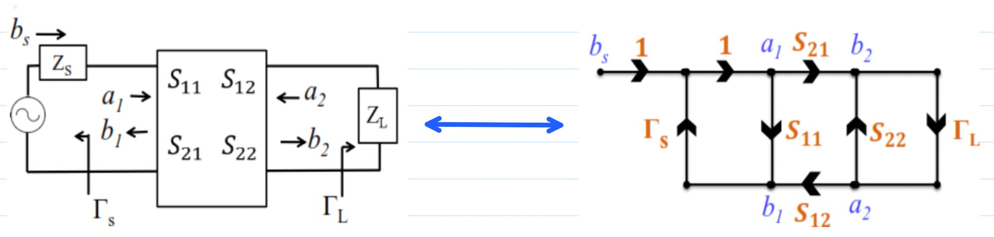
The first equation describes the wave leaving port 1 as a combination of the incident wave at port 1 and the wave incident on port 2. Similarly, the second equation describes the wave leaving port 2. The parameter \(S_{11}\) represents the input reflection characteristic, \(S_{22}\) represents the output reflection characteristic, \(S_{21}\) represents forward transmission, and \(S_{12}\) represents reverse transmission. To analyze the complete amplifier connected between a source and a load, the source and load reflection relationships must now be included with these two-port equations.
5.2 Source and Load Reflection Relationships
At the input port, the source reflects a portion of the wave returning from the amplifier. If \(b_s\) represents the wave supplied by the source, the incident wave \(a_1\) at port 1 consists of the source wave and the wave reflected by the source. Therefore, the source relationship is
\[ a_1=\Gamma_Sb_1+b_s \]
where \(\Gamma_S\) is the reflection coefficient of the source. The source reflection coefficient is defined as
\[ \Gamma_S=\frac{a_1}{b_1} \qquad \text{when } b_s=0 \]
This relationship shows that the signal returning from the amplifier toward the source can be reflected back into the amplifier and therefore forms a feedback path at the input. At the output, the load reflection coefficient relates the wave returning from the load to the wave travelling toward the load. Hence,
\[ a_2=\Gamma_Lb_2 \]
where \(\Gamma_L\) is the load reflection coefficient. The two reflection relationships are therefore
\[ a_1=\Gamma_Sb_1+b_s \]
\[ a_2=\Gamma_Lb_2 \]
These equations, together with the S-parameter equations, form the complete set of relationships required to construct the signal flow graph of the amplifier.
5.3 Forward Paths in the Signal Flow Graph
The source signal \(b_s\) enters the network through the input relation \(a_1=\Gamma_Sb_1+b_s\). From \(a_1\), the forward transmission coefficient \(S_{21}\) produces the output wave \(b_2\). Therefore, the direct forward path from the source \(b_s\) to the output \(b_2\) has a path gain of \(S_{21}\). This is the primary forward path of the amplifier.
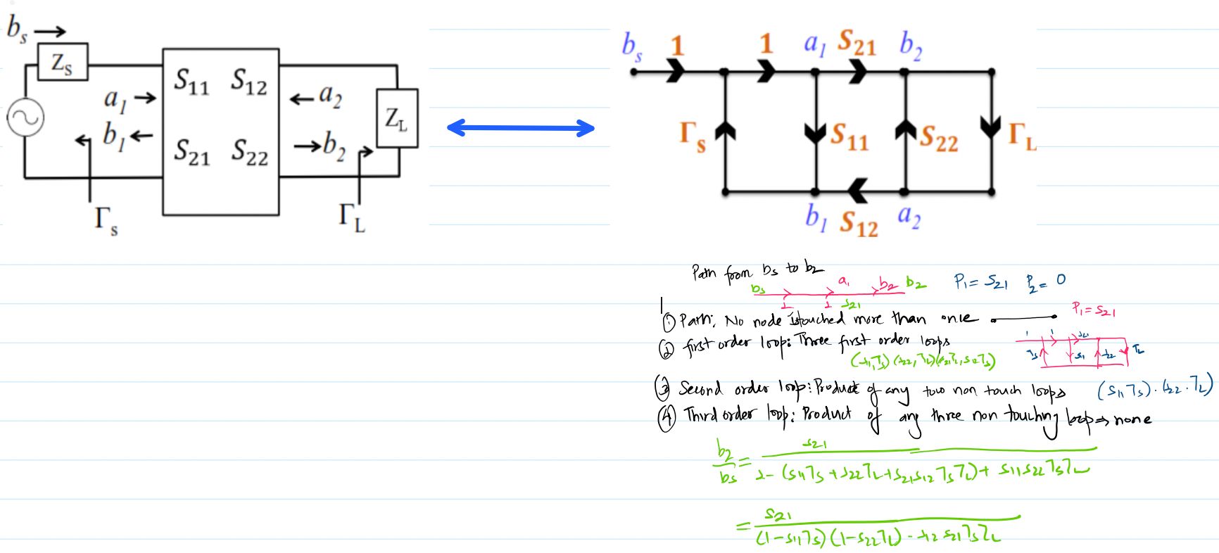
\[ P_1=S_{21} \]
There is also a possible path involving the reverse transmission parameter \(S_{12}\). However, because the source signal enters through \(b_s\) and the output is being considered at \(b_2\), there is no independent direct forward path from \(b_s\) through \(S_{12}\) to \(b_2\). Consequently, the second possible forward path has zero path gain:
\[ P_2=0 \]
Thus, for the transfer from \(b_s\) to \(b_2\), the only nonzero forward path is \(P_1=S_{21}\). The remaining terms in the overall transfer function arise from the feedback loops associated with the source and load reflections and the reverse coupling through \(S_{12}\).
5.4 Individual Loops of the Amplifier Signal Flow Graph
The signal flow graph contains several feedback loops. The first loop begins at \(b_1\), passes through \(S_{11}\), and returns through the source reflection coefficient \(\Gamma_S\). Its loop gain is therefore
\[ L_1=S_{11}\Gamma_S \]
This loop represents the repeated reflection of the signal between the input of the amplifier and the source. A second loop occurs at the output. The signal passes through \(S_{22}\) and then through the load reflection coefficient \(\Gamma_L\), returning to the output node. Its loop gain is
\[ L_2=S_{22}\Gamma_L \]
The third loop includes the forward transmission from the input to the output, reflection from the load, reverse transmission from the output to the input, and reflection from the source. Its loop gain is
\[ L_3=S_{21}\Gamma_LS_{12}\Gamma_S \]
Therefore, the sum of all first-order loops is
\[ \sum L(1) = S_{11}\Gamma_S + S_{22}\Gamma_L + S_{21}S_{12}\Gamma_S\Gamma_L \]
These three loops account for the individual feedback mechanisms present in the complete amplifier network. The first two are associated directly with reflection at the input and output, while the third represents feedback caused by transmission through the amplifier, reflection at the load, reverse transmission, and reflection at the source.
5.5 Non-Touching Loops
Mason’s Signal Flow Rule also requires the identification of loops that do not touch one another. Two loops are considered non-touching when they have no common node. In this amplifier signal flow graph, the input reflection loop \(S_{11}\Gamma_S\) and the output reflection loop \(S_{22}\Gamma_L\) are non-touching. Their product therefore contributes a second-order non-touching loop term:
\[ \sum L(2) = (S_{11}\Gamma_S)(S_{22}\Gamma_L) \]
\[ \sum L(2) = S_{11}S_{22}\Gamma_S\Gamma_L \]
There is no third-order combination of mutually non-touching loops in this signal flow graph. Therefore,
\[ \sum L(3)=0 \]
The distinction between touching and non-touching loops is important because Mason’s rule adds the products of non-touching loops to the denominator with alternating signs. Identifying these loops correctly ensures that all multiple-reflection effects are included in the amplifier transfer function without having to expand the feedback relationships repeatedly by direct substitution.
5.6 Mason’s Signal Flow Rule
Mason’s Signal Flow Rule gives the transfer function between an input node and an output node of a signal flow graph. In its general form, the transfer function is obtained by multiplying each forward-path gain by the determinant associated with the loops that do not touch that path, adding the resulting path contributions, and dividing by the overall graph determinant. The general form can be written as
\[ \text{Transfer Function} = \frac{ P_1\left[1-\sum L(1)^1+\sum L(2)^1-\sum L(3)^1-\cdots\right] + P_2\left[1-\sum L(1)^2+\sum L(2)^2-\sum L(3)^2-\cdots\right] }{ 1-\sum L(1)+\sum L(2)-\sum L(3)+\cdots } \]
Here, \(P_1,P_2,\ldots\) represent the forward-path gains between the input and output nodes. The quantities \(\sum L(1),\sum L(2),\sum L(3)\) represent the sums of first-order, second-order, and third-order combinations of non-touching loops in the complete graph. The superscript associated with a forward path indicates that only loops which do not touch that particular path are included in the corresponding path determinant.
5.7 Application of Mason’s Rule to the Microwave Amplifier
For the microwave amplifier, the only nonzero forward path from \(b_s\) to \(b_2\) is \(P_1=S_{21}\). The second path has \(P_2=0\). The first-order loop sum is
\[ \sum L(1) = S_{11}\Gamma_S + S_{22}\Gamma_L + S_{21}S_{12}\Gamma_S\Gamma_L \]
The second-order non-touching loop sum is
\[ \sum L(2) = S_{11}S_{22}\Gamma_S\Gamma_L \]
and there is no third-order non-touching loop. Substituting these quantities into Mason’s rule gives
\[ \frac{b_2}{b_s} = \frac{ S_{21} }{ 1- \left( S_{11}\Gamma_S + S_{22}\Gamma_L + S_{21}S_{12}\Gamma_S\Gamma_L \right) + S_{11}S_{22}\Gamma_S\Gamma_L } \]
Rearranging the denominator gives
\[ \frac{b_2}{b_s} = \frac{ S_{21} }{ 1-S_{11}\Gamma_S-S_{22}\Gamma_L -S_{21}S_{12}\Gamma_S\Gamma_L +S_{11}S_{22}\Gamma_S\Gamma_L } \]
The denominator can be factored into a more useful form as
\[ \boxed{ \frac{b_2}{b_s} = \frac{ S_{21} }{ (1-S_{11}\Gamma_S)(1-S_{22}\Gamma_L) -S_{21}S_{12}\Gamma_S\Gamma_L } } \]
This is the complete signal transfer relationship between the source wave and the output wave of the microwave amplifier. The denominator contains all of the multiple-reflection and feedback effects associated with the source, load, input reflection, output reflection, forward transmission, and reverse transmission. Mason’s method therefore provides the same physical result obtained through direct S-parameter manipulation, but organizes the different signal paths and feedback mechanisms in a systematic graphical form.
6. Three Cases of Microwave Amplifier Gain
The general transducer power-gain expression can be simplified under specific operating conditions. Three important cases are commonly considered in microwave amplifier analysis: matched transducer power gain, unilateral transducer power gain, and maximum unilateral transducer power gain. Each case applies an additional condition to the general two-port amplifier model. These cases are useful because they progressively simplify the interaction between the source, amplifier, and load and provide practical gain expressions for different amplifier designs.
6.1 Matched Transducer Power Gain
The first case occurs when both the source and load are matched to the reference impedance. Under matched conditions, there is no reflection at either termination, so
\[ \Gamma_S=0 \]
\[ \Gamma_L=0 \]
The general transducer power gain is
\[ G_T= \frac{ |S_{21}|^2 (1-|\Gamma_S|^2) (1-|\Gamma_L|^2) }{ |1-S_{22}\Gamma_L|^2 |1-\Gamma_S\Gamma_{in}|^2 } \]
Substituting \(\Gamma_S=0\) and \(\Gamma_L=0\) gives
\[ G_{tm}=|S_{21}|^2 \]
Therefore, the matched transducer power gain is directly equal to the squared magnitude of the forward transmission coefficient. In a perfectly matched two-port amplifier, the source supplies power without input reflection and the amplifier delivers power to the load without output reflection. This makes \(S_{21}\) a direct measure of the voltage-wave transmission and \(|S_{21}|^2\) the corresponding matched power gain.
6.2 Unilateral Transducer Power Gain
The second case is the unilateral amplifier, for which the reverse transmission from port 2 to port 1 is negligible. This condition is represented by
\[ S_{12}=0 \]
When \(S_{12}=0\), the output of the amplifier no longer feeds back into the input through reverse transmission. The input reflection coefficient therefore reduces to
\[ \Gamma_{in}=S_{11} \]
Similarly, the output reflection coefficient becomes
\[ \Gamma_{out}=S_{22} \]
The general transducer power gain can consequently be written as
\[ G_{tu} = \frac{ |S_{21}|^2 (1-|\Gamma_S|^2) (1-|\Gamma_L|^2) }{ |1-\Gamma_SS_{11}|^2 |1-S_{22}\Gamma_L|^2 } \]
The important feature of this expression is that the source and load matching factors are separated. The input portion of the gain depends on \(S_{11}\) and \(\Gamma_S\), while the output portion depends on \(S_{22}\) and \(\Gamma_L\). Since the reverse transmission coefficient is zero, changing the load does not alter the input reflection coefficient, and changing the source does not alter the output reflection coefficient. This independence makes unilateral analysis considerably simpler than the general bilateral amplifier case.
6.3 Maximum Unilateral Transducer Power Gain
The unilateral transducer gain reaches its maximum value when the source and load are conjugately matched to the input and output of the amplifier. For a unilateral device, \(\Gamma_{in}=S_{11}\) and \(\Gamma_{out}=S_{22}\). Therefore, the conjugate-matching conditions are
\[ \Gamma_S=S_{11}^* \]
\[ \Gamma_L=S_{22}^* \]
The first factor in the unilateral gain expression is then evaluated as
\[ \frac{1-|\Gamma_S|^2} {|1-S_{11}\Gamma_S|^2} = \frac{1-|S_{11}|^2} {|1-S_{11}S_{11}^*|^2} \]
Since \(S_{11}S_{11}^*=|S_{11}|^2\), this becomes
\[ \frac{1-|S_{11}|^2} {(1-|S_{11}|^2)^2} = \frac{1}{1-|S_{11}|^2} \]
Similarly, for the output matching factor,
\[ \frac{1-|\Gamma_L|^2} {|1-S_{22}\Gamma_L|^2} = \frac{1-|S_{22}|^2} {|1-S_{22}S_{22}^*|^2} \]
which gives
\[ \frac{1-|S_{22}|^2} {(1-|S_{22}|^2)^2} = \frac{1}{1-|S_{22}|^2} \]
Substituting both matching factors into the unilateral transducer gain expression gives the maximum unilateral transducer power gain:
\[ \boxed{ G_{tu\,\max} = \frac{|S_{21}|^2} {(1-|S_{11}|^2)(1-|S_{22}|^2)} } \]
This expression represents the maximum power gain obtainable from a unilateral microwave amplifier when both the source and load are conjugately matched. The result shows the three main factors controlling the maximum gain: the forward transmission magnitude \(|S_{21}|^2\), the input reflection coefficient \(S_{11}\), and the output reflection coefficient \(S_{22}\). A strong forward transmission characteristic increases the available gain, while proper source and load matching allows the maximum power transfer to be obtained at the input and output ports.
6.4 Relationship Between the Three Gain Cases
The three gain cases represent progressively more specific operating conditions of the same microwave amplifier. With both ports matched, the transducer gain reduces to \(G_{tm}=|S_{21}|^2\). When the amplifier is unilateral, the reverse transmission coefficient becomes zero and the transducer gain separates into independent input and output matching factors, giving \(G_{tu}\). Finally, when the unilateral amplifier is conjugately matched at both ports, these matching factors reach their maximum values and the gain becomes \(G_{tu\,\max}\). These expressions provide a useful progression from the directly measurable matched gain to the more detailed gain available when source and load matching are included, and finally to the maximum gain obtainable under ideal unilateral conjugate-matching conditions.
Cases
-
If \(\Gamma_S = 0\) and \(\Gamma_L = 0\), the input and output are matched for zero reflection. Such a special case of Transducer Gain can be represented as
\[ G_T = \frac{|S_{21}|^2 \times (1-0)(1-0)} {(1-0)(1-0)} = |S_{21}|^2 \]
-
Another special case is Unilateral Transducer, when \(S_{12}=0\). In this case, transmission takes place only in one direction.
\[ \Gamma_{in} = \frac{V_1^-}{V_1^+} = S_{11} + \frac{S_{12}S_{21}\Gamma_L} {1-S_{22}\Gamma_L} = S_{11}+0 = S_{11} \]
\[ \Gamma_{out} = \frac{V_2^-}{V_2^+} = S_{22} + \frac{S_{12}S_{21}\Gamma_S} {1-S_{11}\Gamma_S} = S_{22} \]
Then,
\[ G_T = \frac{ |S_{21}|^2 (1-|\Gamma_S|^2) (1-|\Gamma_L|^2) }{ |1-S_{11}\Gamma_S|^2 |1-S_{22}\Gamma_L|^2 } \]
\(G_T\) can also be written as
\[ G_T = \left( \frac{1-|\Gamma_S|^2} {|1-\Gamma_S\Gamma_{in}|^2} \right) \times |S_{21}|^2 \times \left( \frac{1-|\Gamma_L|^2} {|1-S_{22}\Gamma_L|^2} \right) \]
\[ \underbrace{\hspace{2.2cm}}_{G_S} \quad \underbrace{\hspace{1.2cm}}_{G_0} \quad \underbrace{\hspace{2.5cm}}_{G_L} \]