Microwave Amplifier Stability
Microwave Amplifier Stability: Unconditional and Conditional Stability
1. Introduction to Microwave Amplifier Stability
The stability of a microwave amplifier is one of the most important considerations in the design and analysis of any high-frequency transistor amplifier. A microwave amplifier is designed to provide controlled amplification of an input signal over a specified frequency range, but under certain source and load conditions, the same active device can develop unwanted oscillations instead of producing stable amplification. For this reason, stability must be considered not only at the intended operating frequency but across the complete frequency range in which the amplifier may encounter significant signals or feedback conditions. An amplifier that becomes unstable within its operating band cannot provide the intended linear amplification, while instability outside the desired band can also lead to unwanted radiation, interference, or oscillatory behavior at other frequencies.
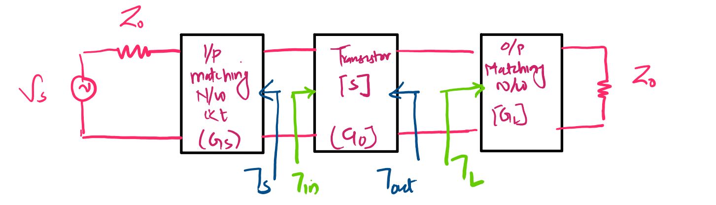
In a microwave transistor amplifier, stability is closely related to the interaction between the transistor and the source and load impedances connected to its input and output ports. Unlike a passive network, an active transistor can provide power to the surrounding network. If the input or output network presents an effective negative real resistance to the transistor, the circuit can potentially sustain an oscillation. Therefore, the stability of the complete amplifier depends not only on the intrinsic properties of the transistor but also on the impedances presented by the source and load. Since microwave circuits are commonly analyzed using scattering parameters and reflection coefficients, these stability conditions can be conveniently expressed in terms of the magnitudes of the input and output reflection coefficients.
1.1 Relationship Between Negative Resistance and Reflection Coefficient
Oscillation is possible when the input or output port of an active microwave network exhibits a negative real resistance. Physically, a negative resistance means that the active device can supply energy to the surrounding circuit rather than simply absorbing energy from it. If the feedback and impedance conditions are appropriate, this supplied energy can compensate for the losses in the circuit and allow an oscillating signal to build up. In terms of reflection coefficients, this behavior is associated with a reflection coefficient magnitude greater than unity at the corresponding port.
The input port can exhibit a potentially unstable condition when the magnitude of its input reflection coefficient satisfies:
\[ \left|\Gamma_{in}\right|>1 \]
Similarly, the output port can exhibit a potentially unstable condition when the magnitude of its output reflection coefficient satisfies:
\[ \left|\Gamma_{out}\right|>1 \]
These conditions provide an intuitive way to understand the possibility of oscillation. The reflection coefficient represents the ratio of the reflected wave to the incident wave at a port. When its magnitude is greater than unity, the reflected wave has a greater magnitude than the incident wave under the relevant power-wave convention. In an active device, this does not violate energy conservation because the additional energy can be supplied by the transistor's DC bias source. The active device is effectively providing energy to the microwave network, and if the circuit conditions allow the returned signal to reinforce itself, sustained oscillation can occur.
1.1.1 Physical Meaning of \(\left|\Gamma\right|>1\)
For a passive network, the magnitude of the reflection coefficient is normally less than or equal to unity because a passive network cannot generate additional signal power. An active microwave transistor is different because it can transfer energy from its DC power supply into the RF signal. Consequently, an active two-port can exhibit an input or output reflection coefficient whose magnitude exceeds unity for certain source or load conditions. Such a condition indicates that the corresponding port can potentially present a negative resistance and therefore participate in oscillation.
The condition \(\left|\Gamma\right|>1\) should therefore be interpreted as an indication of potential instability rather than as a statement that oscillation must occur under every possible circuit condition. The actual behavior depends on the complete feedback path and on the source and load impedances connected to the transistor. Stability analysis determines whether passive source and load impedances can produce these potentially unstable conditions and whether the amplifier remains stable for all permissible passive terminations.
1.2 Unconditional Stability
Unconditional stability means that the microwave amplifier remains stable for every possible passive source and load impedance. In reflection-coefficient terms, passive source and load impedances correspond to points inside the unit Smith Chart, for which \(\left|\Gamma_S\right|<1\) and \(\left|\Gamma_L\right|<1\). An amplifier is unconditionally stable when the input and output reflection coefficients remain less than unity in magnitude for all such passive terminations.
The conditions for unconditional stability can therefore be expressed as:
\[ \left|\Gamma_{in}\right|<1 \]
\[ \left|\Gamma_{out}\right|<1 \]
These conditions must remain satisfied for all passive values of the source and load reflection coefficients within the entire Smith Chart. In other words, there should be no passive source or load impedance that can cause either port to enter the potentially unstable region. This is an important characteristic in practical microwave amplifier design because it means that the amplifier does not rely on one particular source or load impedance to remain stable.
An unconditionally stable transistor therefore provides a much more predictable basis for amplifier design. The designer can select appropriate input and output matching networks to obtain the required gain, noise performance, bandwidth, or impedance transformation without encountering a passive termination that causes the active device to become unstable. Stability is still frequency dependent and must be evaluated over the relevant frequency range, but at a given frequency the unconditional-stability condition covers the complete range of passive source and load terminations.
1.3 Conditional Stability
Conditional stability occurs when the amplifier remains stable only for a certain range of passive source and load impedances. In this situation, some passive terminations result in stable operation, while other passive terminations can cause the input or output reflection coefficient magnitude to exceed unity. The device is therefore sometimes described as potentially unstable because its stability depends on the particular source and load impedances connected to it.
For a conditionally stable amplifier, the conditions \(\left|\Gamma_{in}\right|<1\) and \(\left|\Gamma_{out}\right|<1\) are satisfied only within particular regions of the permissible source and load reflection-coefficient planes. The designer must therefore select the input and output matching networks carefully so that the actual operating points remain inside the stable regions. This makes stability analysis an important part of the matching-network design process rather than a separate consideration performed only after the amplifier has been designed.
The distinction between unconditional and conditional stability is particularly useful when working with the Smith Chart. In the unconditional case, every passive source and load impedance represented within the Smith Chart produces stable operation. In the conditional case, the Smith Chart is divided into stable and potentially unstable regions, and the designer must identify the appropriate region before selecting the source and load matching impedances.
1.4 Frequency Dependence of Amplifier Stability
The stability of a microwave amplifier is generally frequency dependent. The S-parameters of a transistor vary with frequency, and the input and output matching networks also exhibit frequency-dependent impedance characteristics. Consequently, an amplifier that is stable at its design frequency may not necessarily remain stable at frequencies above or below the design frequency. This is particularly important in wideband microwave amplifier design, where the transistor may encounter a wide range of impedances and feedback conditions across the operating spectrum.
For example, a transistor may have acceptable values of \(\left|\Gamma_{in}\right|\) and \(\left|\Gamma_{out}\right|\) at its nominal operating frequency while developing a potentially unstable condition at another frequency. Therefore, checking stability at only one frequency does not by itself guarantee stability across the entire frequency range. The frequency response of the transistor S-parameters, together with the frequency-dependent behavior of the input and output matching networks, must be considered when evaluating the complete amplifier.
This frequency dependence also explains why stability analysis is critical even outside the amplifier's intended signal band. An unwanted oscillation at another frequency can interfere with the amplifier's operation, introduce unwanted spectral components, reduce linearity, or potentially cause interference with other systems. A complete microwave amplifier design therefore considers stability over the relevant frequency range rather than treating stability as a single-frequency property.
1.5 Importance of Stability in Microwave Amplifier Design
Stability must be guaranteed as part of the overall microwave amplifier design because an unstable amplifier cannot reliably provide the intended amplification. The source and load matching networks are normally designed to transform impedances for a particular gain or power-transfer requirement, but these same networks also influence the feedback conditions seen by the transistor. A matching network that improves gain at one frequency or operating point can alter the input or output reflection coefficient enough to move the amplifier toward an unstable region. Stability must therefore be considered together with gain and impedance matching rather than treated as an independent final check.
The fundamental distinction is that an unconditionally stable amplifier remains stable for every passive source and load impedance, whereas a conditionally stable amplifier remains stable only for specified ranges of passive source and load impedances. The reflection-coefficient conditions provide the starting point for identifying these behaviors. When the input or output reflection coefficient magnitude reaches unity, a stability boundary is encountered, and when it exceeds unity, the corresponding port can become potentially unstable.
For a two-port microwave transistor, these stability conditions can be evaluated from its S-parameters and the source and load reflection coefficients. The resulting boundaries can be represented graphically on the Smith Chart as stability circles. These circles identify the regions of source or load reflection coefficients associated with stable and potentially unstable operation. The detailed construction and mathematical derivation of these stability circles form the next stage of microwave amplifier stability analysis.
Stability Conditions and Stability Circles of a Microwave Amplifier
2. Stability Conditions and Stability Circles
The stability of a microwave amplifier can be analyzed quantitatively using the scattering parameters of the transistor together with the source and load reflection coefficients. For a general two-port transistor, the input and output reflection coefficients are not determined only by \(S_{11}\) and \(S_{22}\), respectively. Because a practical transistor may have reverse transmission represented by \(S_{12}\), the termination connected to one port can influence the reflection coefficient observed at the other port. Therefore, the source and load matching networks play an important role in determining the stability of the complete amplifier.
The input reflection coefficient \(\Gamma_{in}\) describes the reflection seen looking into the input port of the transistor when the output port is terminated by the load reflection coefficient \(\Gamma_L\). For a general two-port network, it is given by:
\[ \Gamma_{in} = S_{11} + \frac{S_{12}S_{21}\Gamma_L} {1-S_{22}\Gamma_L} \]
This expression shows that \(\Gamma_{in}\) depends not only on the transistor's input reflection coefficient \(S_{11}\), but also on the load reflection coefficient \(\Gamma_L\). The second term represents the effect of reverse and forward transmission through the transistor and the reflection produced by the load. Consequently, changing the load impedance can change the effective input reflection coefficient of the transistor and therefore influence amplifier stability.
Similarly, the output reflection coefficient \(\Gamma_{out}\) describes the reflection seen looking into the output port when the input port is terminated by the source reflection coefficient \(\Gamma_S\). For a general two-port transistor, it is expressed as:
\[ \Gamma_{out} = S_{22} + \frac{S_{12}S_{21}\Gamma_S} {1-S_{11}\Gamma_S} \]
The output reflection coefficient therefore depends on both the intrinsic output reflection parameter \(S_{22}\) and the source termination connected to the input port. This relationship is especially important for a potentially unstable transistor because a change in the source impedance can alter the effective output reflection coefficient and move the amplifier between stable and potentially unstable operating regions.
2.1 Input Stability Condition
From the stability principle introduced in the previous section, a microwave amplifier is stable at its input when the magnitude of the input reflection coefficient is less than unity. Therefore, the input stability condition is:
\[ \left|\Gamma_{in}\right|<1 \]
Substituting the general expression for \(\Gamma_{in}\), the condition becomes:
\[ \left| S_{11} + \frac{S_{12}S_{21}\Gamma_L} {1-S_{22}\Gamma_L} \right| <1 \]
This inequality defines the stable condition in terms of the possible load reflection coefficient \(\Gamma_L\). For a passive load, \(\left|\Gamma_L\right|<1\), so the relevant values of \(\Gamma_L\) lie within the Smith Chart. Some of these load reflection coefficients may produce a stable input condition, while others may produce \(\left|\Gamma_{in}\right|>1\) and therefore a potentially unstable condition.
The boundary between these two regions occurs when the magnitude of the input reflection coefficient is exactly equal to unity. Hence, the input stability boundary is obtained from:
\[ \left| S_{11} + \frac{S_{12}S_{21}\Gamma_L} {1-S_{22}\Gamma_L} \right| =1 \]
This equation describes the set of load reflection coefficients for which the input reflection coefficient has unit magnitude. When represented in the complex \(\Gamma_L\) plane, this boundary forms a circle under the usual two-port stability-circle formulation. It is therefore called the output stability circle, because it is plotted in the load reflection-coefficient plane and identifies the load terminations that establish the boundary of input stability.
2.2 Output Stability Condition
The corresponding stability condition at the output requires the magnitude of the output reflection coefficient to remain less than unity. Thus, the output stability condition is:
\[ \left|\Gamma_{out}\right|<1 \]
Using the general expression for the output reflection coefficient gives:
\[ \left| S_{22} + \frac{S_{12}S_{21}\Gamma_S} {1-S_{11}\Gamma_S} \right| <1 \]
This condition depends on the source reflection coefficient \(\Gamma_S\). Therefore, different passive source impedances can produce different values of \(\left|\Gamma_{out}\right|\). If the source termination is selected from a region in which \(\left|\Gamma_{out}\right|<1\), the output port satisfies the stability requirement. If the source termination produces \(\left|\Gamma_{out}\right|>1\), the amplifier can become potentially unstable.
The boundary between the stable and potentially unstable regions is obtained by setting the magnitude of the output reflection coefficient equal to unity:
\[ \left| S_{22} + \frac{S_{12}S_{21}\Gamma_S} {1-S_{11}\Gamma_S} \right| =1 \]
This equation defines a circle in the complex \(\Gamma_S\) plane. Because the circle is represented in the source reflection-coefficient plane, it is referred to as the input stability circle. It identifies the source terminations for which the output of the transistor is exactly at the stability boundary.
2.3 Stability Boundary and Stability Circles
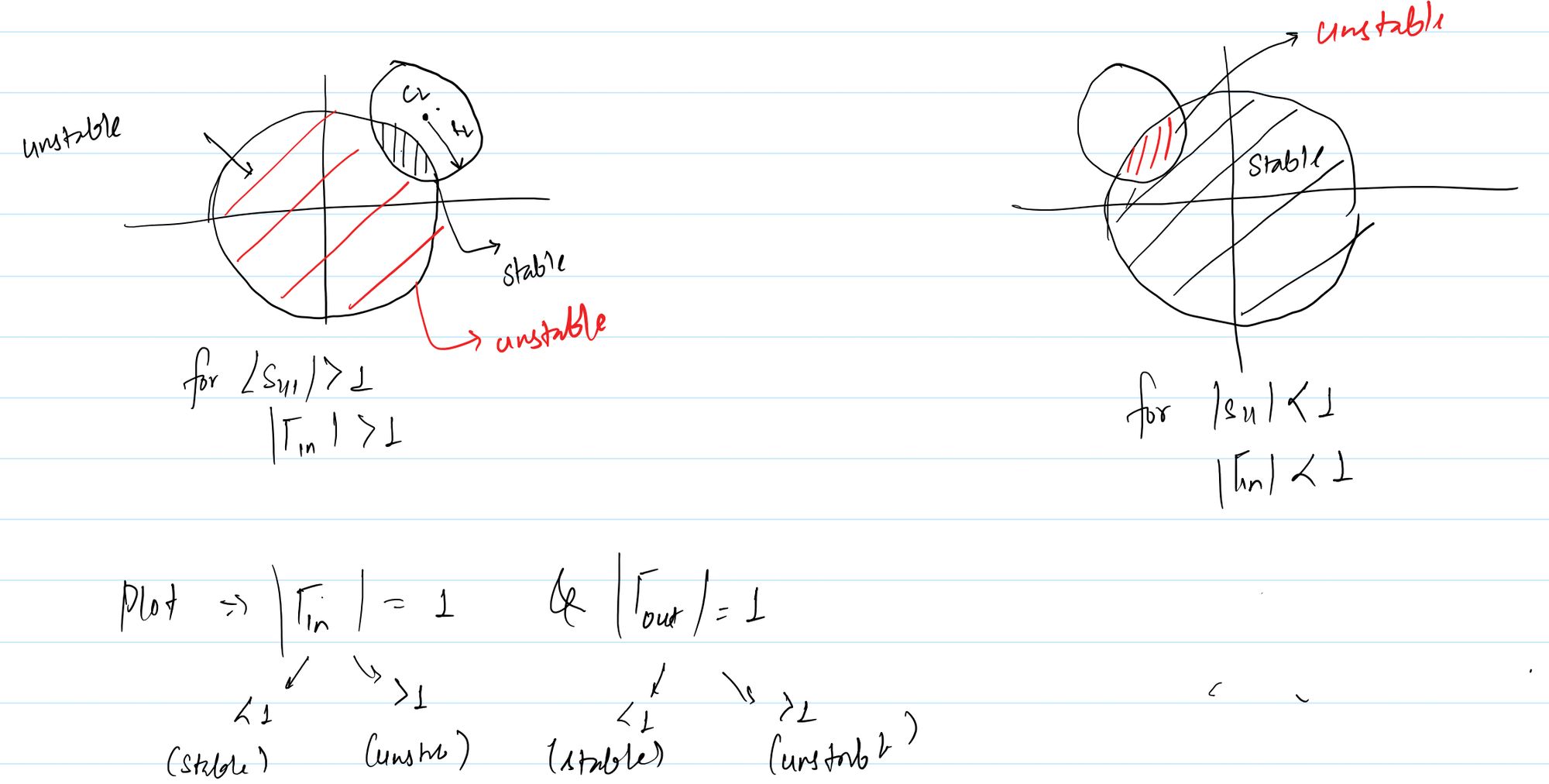
The equality condition \(\left|\Gamma\right|=1\) is important because it represents the boundary between stable and potentially unstable behavior. Inside one region of the reflection-coefficient plane, the corresponding reflection coefficient may satisfy \(\left|\Gamma\right|<1\), while in another region it may satisfy \(\left|\Gamma\right|>1\). The exact stable region depends on the transistor S-parameters and must be determined from the particular stability circle and an appropriate test point.
The two stability-boundary equations can therefore be written together as:
\[ \left| S_{11} + \frac{S_{12}S_{21}\Gamma_L} {1-S_{22}\Gamma_L} \right| =1 \]
\[ \left| S_{22} + \frac{S_{12}S_{21}\Gamma_S} {1-S_{11}\Gamma_S} \right| =1 \]
These equations generate the two fundamental stability circles used in microwave amplifier analysis. The first equation is associated with the load reflection coefficient \(\Gamma_L\), so it produces the output stability circle. The second equation is associated with the source reflection coefficient \(\Gamma_S\), so it produces the input stability circle. Together, these circles provide a graphical method for investigating how source and load terminations influence the stability of a two-port microwave transistor.
2.4 Output Stability Circle
The output stability circle is plotted on the Smith Chart whose complex coordinate is the load reflection coefficient \(\Gamma_L\). Every point on this circle satisfies the condition \(\left|\Gamma_{in}\right|=1\). The circle therefore represents the boundary between load impedances that result in different input stability conditions. When the load reflection coefficient is selected on one side of the circle, the transistor may satisfy \(\left|\Gamma_{in}\right|<1\), whereas the other side may correspond to \(\left|\Gamma_{in}\right|>1\).
It is important to note that the circle itself does not automatically identify which side is stable. The stable region must be determined by evaluating a suitable test point, commonly a simple point such as \(\Gamma_L=0\), and checking the resulting value of \(\left|\Gamma_{in}\right|\). Once the stable side has been identified, the Smith Chart can be used to select an appropriate load matching condition that keeps the amplifier within the stable region.
2.5 Input Stability Circle
The input stability circle is plotted on the Smith Chart whose complex coordinate is the source reflection coefficient \(\Gamma_S\). Every point on this circle satisfies the condition \(\left|\Gamma_{out}\right|=1\). The circle therefore separates source reflection-coefficient regions associated with different output stability conditions.
As with the output stability circle, the stable side of the input stability circle is not determined merely by looking at the circle. A test point can be selected and substituted into the expression for \(\Gamma_{out}\) to determine whether that region satisfies \(\left|\Gamma_{out}\right|<1\) or \(\left|\Gamma_{out}\right|>1\). This allows the designer to identify the permissible source impedance region before designing the input matching network.
2.6 Stability Circles on the Smith Chart
The Smith Chart provides a convenient graphical representation of the complex source and load reflection coefficients. Since passive impedances correspond to points within the unit circle of the reflection-coefficient plane, stability circles can be drawn over the Smith Chart to determine which passive terminations produce stable or potentially unstable operation. The position and size of a stability circle are determined by the transistor's S-parameters at the frequency under consideration.
For a conditionally stable transistor, a stability circle may pass through the Smith Chart and divide the available passive impedance region into stable and potentially unstable portions. The designer can then select the source or load matching impedance from the stable region. This graphical approach is particularly useful because it allows stability requirements to be considered together with impedance matching, gain, and other design objectives on the same reflection-coefficient plane.
The output stability circle uses \(\Gamma_L\) as its complex-plane variable, whereas the input stability circle uses \(\Gamma_S\). This distinction is important when interpreting a stability-circle diagram. The output stability circle determines how the choice of load termination affects input stability, while the input stability circle determines how the choice of source termination affects output stability. Both are consequences of the two-way coupling represented by the transistor's S-parameters.
2.7 Interpretation of Stable and Potentially Unstable Regions
The stability circles are boundaries rather than automatic indicators of the stable region. A point located exactly on a stability circle satisfies the limiting condition \(\left|\Gamma_{in}\right|=1\) or \(\left|\Gamma_{out}\right|=1\). Points on one side of the circle satisfy the stable inequality, while points on the other side can satisfy the potentially unstable inequality. The appropriate region must therefore be identified from the actual S-parameter values rather than assumed solely from the geometric position of the circle.
For amplifier design, the practical objective is to ensure that the selected source and load reflection coefficients remain within regions where both input and output stability requirements are satisfied. This means that the input matching network should present a source reflection coefficient within an acceptable stable region, while the output matching network should present a load reflection coefficient within its corresponding stable region. When the transistor is unconditionally stable, every passive source and load termination satisfies the required stability conditions. When the transistor is conditionally stable, however, the matching networks must be designed with explicit consideration of the stability-circle boundaries.
The stability-circle equations provide the foundation for this graphical analysis. By converting the conditions \(\left|\Gamma_{in}\right|=1\) and \(\left|\Gamma_{out}\right|=1\) into circle equations, the effects of source and load terminations can be visualized directly on the Smith Chart. The next stage is to mathematically manipulate these boundary equations into the standard circle form and obtain the center and radius of the input and output stability circles.
Derivation of Input and Output Stability Circle Equations
3. Derivation of Input and Output Stability Circle Equations
The stability circles of a microwave amplifier are obtained by converting the stability-boundary conditions into the standard equation of a circle in the complex reflection-coefficient plane. This mathematical derivation is important because the resulting center and radius allow the stability boundary to be plotted directly on a Smith Chart. For a general two-port transistor, the output stability circle is obtained in the \(\Gamma_L\) plane from the condition \(\left|\Gamma_{in}\right|=1\), while the input stability circle is obtained in the \(\Gamma_S\) plane from the condition \(\left|\Gamma_{out}\right|=1\).
The derivation begins with the general input reflection coefficient and output reflection coefficient introduced previously. The algebra becomes considerably simpler by introducing the determinant of the transistor's S-matrix, denoted by \(\Delta\). For a two-port network, this determinant is defined as:
\[ \Delta=S_{11}S_{22}-S_{12}S_{21} \]
The quantity \(\Delta\) combines the four scattering parameters into a single parameter and naturally appears when the stability-boundary equation is simplified. We first derive the output stability circle in detail and then obtain the input stability circle using the corresponding interchange of input and output quantities.
3.1 Output Stability Circle Boundary
The output stability circle is associated with the load reflection coefficient \(\Gamma_L\). Its boundary is obtained by setting the magnitude of the input reflection coefficient equal to unity. Starting with:
\[ \left|\Gamma_{in}\right|=1 \]
and substituting the general expression for \(\Gamma_{in}\), we obtain:
\[ \left| S_{11} + \frac{S_{12}S_{21}\Gamma_L} {1-S_{22}\Gamma_L} \right| =1 \]
To remove the fraction, multiply the expression inside the magnitude by \(1-S_{22}\Gamma_L\). Because the magnitude of a ratio is the ratio of the magnitudes, the boundary condition can be written as:
\[ \left| S_{11}(1-S_{22}\Gamma_L) + S_{12}S_{21}\Gamma_L \right| = \left| 1-S_{22}\Gamma_L \right| \]
Expanding the expression on the left gives:
\[ \left| S_{11} - S_{11}S_{22}\Gamma_L + S_{12}S_{21}\Gamma_L \right| = \left| 1-S_{22}\Gamma_L \right| \]
Using the definition of \(\Delta\), we have:
\[ S_{11}S_{22}-S_{12}S_{21}=\Delta \]
Therefore, the terms containing \(\Gamma_L\) on the left-hand side can be combined:
\[ -S_{11}S_{22}\Gamma_L + S_{12}S_{21}\Gamma_L = -\Delta\Gamma_L \]
Hence, the stability-boundary equation becomes:
\[ \left| S_{11}-\Delta\Gamma_L \right| = \left| 1-S_{22}\Gamma_L \right| \]
This compact form is the starting point for converting the stability boundary into the standard circle equation.
3.2 Expansion of the Magnitude-Squared Terms
Since both sides of the equation are nonnegative real quantities, the magnitudes can be squared without changing the equality. Thus:
\[ \left| S_{11}-\Delta\Gamma_L \right|^2 = \left| 1-S_{22}\Gamma_L \right|^2 \]
For any complex quantities \(A\) and \(B\), the magnitude squared of their difference is:
\[ |A-B|^2 = (A-B)(A^*-B^*) \]
Applying this relation to the left-hand side gives:
\[ \left| S_{11}-\Delta\Gamma_L \right|^2 = (S_{11}-\Delta\Gamma_L) (S_{11}^*-\Delta^*\Gamma_L^*) \]
Multiplying the two factors produces:
\[ |S_{11}|^2 - S_{11}\Delta^*\Gamma_L^* - S_{11}^*\Delta\Gamma_L + |\Delta|^2|\Gamma_L|^2 \]
Similarly, the right-hand side becomes:
\[ \left| 1-S_{22}\Gamma_L \right|^2 = (1-S_{22}\Gamma_L) (1-S_{22}^*\Gamma_L^*) \]
Expanding this expression gives:
\[ 1 - S_{22}\Gamma_L - S_{22}^*\Gamma_L^* + |S_{22}|^2|\Gamma_L|^2 \]
Equating the two expanded expressions gives:
\[ |S_{11}|^2 - S_{11}\Delta^*\Gamma_L^* - S_{11}^*\Delta\Gamma_L + |\Delta|^2|\Gamma_L|^2 = 1 - S_{22}\Gamma_L - S_{22}^*\Gamma_L^* + |S_{22}|^2|\Gamma_L|^2 \]
3.3 Collecting the \(\Gamma_L\) and \(\Gamma_L^*\) Terms
Move all terms to the left-hand side and collect the terms according to their dependence on \(\Gamma_L\), \(\Gamma_L^*\), and \(|\Gamma_L|^2\). The result is:
\[ \left(|\Delta|^2-|S_{22}|^2\right)|\Gamma_L|^2 + \left(S_{22}-S_{11}^*\Delta\right)\Gamma_L + \left(S_{22}^*-S_{11}\Delta^*\right)\Gamma_L^* + |S_{11}|^2-1 = 0 \]
Notice that the coefficients of \(\Gamma_L\) and \(\Gamma_L^*\) are complex conjugates of each other. This is exactly the structure expected for a circle equation in the complex plane. To make this structure clearer, define:
\[ A=|\Delta|^2-|S_{22}|^2 \]
\[ B=S_{22}-S_{11}^*\Delta \]
\[ B^*=S_{22}^*-S_{11}\Delta^* \]
\[ C=|S_{11}|^2-1 \]
The equation can then be written in the compact form:
\[ A|\Gamma_L|^2+B\Gamma_L+B^*\Gamma_L^*+C=0 \]
The purpose of introducing these quantities is only to simplify the completion-of-the-square operation. The final stability-circle parameters will be expressed entirely in terms of the original S-parameters and \(\Delta\).
3.4 Completing the Square for the Output Stability Circle
Divide the equation by \(A\), assuming \(A\neq0\):
\[ |\Gamma_L|^2 + \frac{B}{A}\Gamma_L + \frac{B^*}{A}\Gamma_L^* + \frac{C}{A} = 0 \]
The first three terms can be converted into the squared magnitude of a complex quantity. For a complex number \(C_L\), the identity
\[ |\Gamma_L-C_L|^2 = |\Gamma_L|^2 - C_L^*\Gamma_L - C_L\Gamma_L^* + |C_L|^2 \]
can be used to identify the center of the circle. Comparing this identity with the normalized stability equation gives:
\[ -C_L^*=\frac{B}{A} \]
Therefore:
\[ C_L=-\frac{B^*}{A} \]
Substituting \(B=S_{22}-S_{11}^*\Delta\) and \(A=|\Delta|^2-|S_{22}|^2\), we obtain:
\[ C_L = \frac{S_{22}^*-S_{11}\Delta^*} {|S_{22}|^2-|\Delta|^2} \]
The numerator can equivalently be written in the compact conjugate form:
\[ C_L= \frac{(S_{22}-\Delta S_{11}^{*})^{*}} {|S_{22}|^2-|\Delta|^2} \]
Thus, the center of the output stability circle is:
\[ \boxed{ C_L= \frac{(S_{22}-\Delta S_{11}^{*})^{*}} {|S_{22}|^2-|\Delta|^2} } \]
The remaining constant terms determine the radius. After completing the square, the equation takes the form:
\[ |\Gamma_L-C_L|^2=R_L^2 \]
The radius is obtained from the constant portion of the completed-square expression. After substituting the definitions of \(A\), \(B\), and \(C\), the resulting expression simplifies using the identity associated with the determinant \(\Delta=S_{11}S_{22}-S_{12}S_{21}\). The final radius is:
\[ \boxed{ R_L= \left| \frac{S_{12}S_{21}} {|S_{22}|^2-|\Delta|^2} \right| } \]
Therefore, the complete output stability circle is:
\[ \boxed{ |\Gamma_L-C_L|=R_L } \]
where \(C_L\) and \(R_L\) are given by the expressions above. This is the standard circle equation in the complex \(\Gamma_L\) plane.
3.5 Physical Meaning of the Output Stability Circle Center and Radius
The quantity \(C_L\) represents the center of the output stability circle in the load reflection-coefficient plane. Because \(\Gamma_L\) is generally complex, the center is also a complex number and specifies the location of the circle relative to the center of the Smith Chart. Its value is determined entirely by the transistor's S-parameters at the frequency being analyzed.
The quantity \(R_L\) represents the radius of the output stability circle. Every load reflection coefficient lying exactly \(R_L\) away from \(C_L\) satisfies the boundary condition \(\left|\Gamma_{in}\right|=1\). Consequently, the circle separates regions in the \(\Gamma_L\) plane that produce different input stability conditions. The circle itself is a boundary and does not by itself identify which side is stable; a test point must be used to determine whether a particular region satisfies \(\left|\Gamma_{in}\right|<1\).
3.6 Input Stability Circle Derivation
The input stability circle is derived in an analogous manner from the output stability condition. The boundary is defined by:
\[ \left|\Gamma_{out}\right|=1 \]
Substituting the general expression for \(\Gamma_{out}\) gives:
\[ \left| S_{22} + \frac{S_{12}S_{21}\Gamma_S} {1-S_{11}\Gamma_S} \right| =1 \]
Multiplying through by the magnitude of the denominator produces:
\[ \left| S_{22}(1-S_{11}\Gamma_S) + S_{12}S_{21}\Gamma_S \right| = \left| 1-S_{11}\Gamma_S \right| \]
Expanding the expression inside the left-hand magnitude gives:
\[ \left| S_{22} - S_{22}S_{11}\Gamma_S + S_{12}S_{21}\Gamma_S \right| = \left| 1-S_{11}\Gamma_S \right| \]
Using the definition of \(\Delta\), the coefficient of \(\Gamma_S\) becomes \(-\Delta\), so the boundary condition reduces to:
\[ \left| S_{22}-\Delta\Gamma_S \right| = \left| 1-S_{11}\Gamma_S \right| \]
Squaring both sides and expanding the magnitude-squared terms gives:
\[ \left| S_{22}-\Delta\Gamma_S \right|^2 = \left| 1-S_{11}\Gamma_S \right|^2 \]
After expanding, collecting the \(\Gamma_S\), \(\Gamma_S^*\), and \(|\Gamma_S|^2\) terms, and completing the square in exactly the same manner as for the output stability circle, the equation can be converted to:
\[ |\Gamma_S-C_S|=R_S \]
The center of the input stability circle is:
\[ \boxed{ C_S= \frac{(S_{11}-\Delta S_{22}^{*})^{*}} {|S_{11}|^2-|\Delta|^2} } \]
The corresponding radius is:
\[ \boxed{ R_S= \left| \frac{S_{12}S_{21}} {|S_{11}|^2-|\Delta|^2} \right| } \]
Thus, the complete input stability-circle equation is:
\[ \boxed{ |\Gamma_S-C_S|=R_S } \]
3.7 Physical Meaning of the Input Stability Circle Center and Radius
The complex quantity \(C_S\) specifies the center of the input stability circle in the source reflection-coefficient plane. It determines where the boundary is positioned on the Smith Chart. The radius \(R_S\) specifies the distance from this center to every point on the stability boundary. Every source reflection coefficient satisfying \(|\Gamma_S-C_S|=R_S\) produces the limiting condition \(\left|\Gamma_{out}\right|=1\).
The input stability circle therefore divides the source reflection-coefficient plane into regions having different output stability behavior. As with the output stability circle, the stable side cannot be identified from the circle equation alone. A convenient test point, such as \(\Gamma_S=0\), can be substituted into the original output reflection-coefficient expression to determine whether the selected region satisfies \(\left|\Gamma_{out}\right|<1\).
3.8 Final Stability Circle Equations
The mathematical derivation produces two standard stability-circle equations. The output stability circle is represented in the load reflection-coefficient plane and is obtained from the input stability boundary:
\[ \boxed{ |\Gamma_L-C_L|=R_L } \]
\[ \boxed{ C_L= \frac{(S_{22}-\Delta S_{11}^{*})^{*}} {|S_{22}|^2-|\Delta|^2} } \]
\[ \boxed{ R_L= \left| \frac{S_{12}S_{21}} {|S_{22}|^2-|\Delta|^2} \right| } \]
The input stability circle is represented in the source reflection-coefficient plane and is obtained from the output stability boundary:
\[ \boxed{ |\Gamma_S-C_S|=R_S } \]
\[ \boxed{ C_S= \frac{(S_{11}-\Delta S_{22}^{*})^{*}} {|S_{11}|^2-|\Delta|^2} } \]
\[ \boxed{ R_S= \left| \frac{S_{12}S_{21}} {|S_{11}|^2-|\Delta|^2} \right| \]
These equations show that the locations and sizes of the stability circles are controlled by the transistor's scattering parameters. In particular, the product \(S_{12}S_{21}\) appears in the numerator of both radii, showing the role of two-port transmission coupling in the stability boundary. The determinant \(\Delta\) also influences both the circle center and radius and therefore cannot generally be neglected in a bilateral transistor.
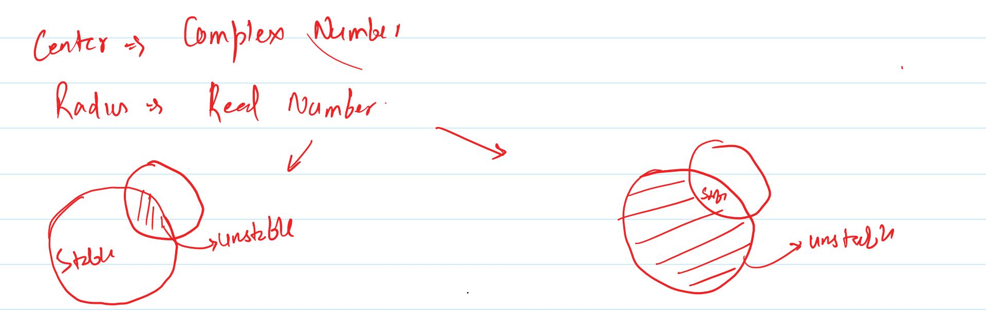
At a given operating frequency, the calculated \(C_L\) and \(R_L\) can be used to plot the output stability circle on the \(\Gamma_L\) Smith Chart, while \(C_S\) and \(R_S\) can be used to plot the input stability circle on the \(\Gamma_S\) Smith Chart. Once these circles are plotted, a test point can be used to identify the stable region. The resulting graphical information is particularly useful for a conditionally stable transistor, where the choice of source and load matching networks must be restricted to appropriate regions of the Smith Chart.
Unconditional Stability Tests: K-Delta and Mu Tests for Microwave Amplifiers
4. Unconditional Stability Tests: K-Delta and Mu Tests
The stability circles derived in the previous sections provide a graphical method for determining the source and load reflection-coefficient regions that produce stable operation. However, when the main objective is simply to determine whether a microwave transistor is unconditionally stable, it is often more convenient to use analytical stability tests. Two widely used criteria are the Rollet stability factor \(K\) with the determinant \(\Delta\) and the \(\mu\)-test. These tests use the transistor's scattering parameters directly and can determine unconditional stability without requiring the stability circles to be plotted first.
The K-Delta test is based on two quantities, \(K\) and \(\Delta\), while the \(\mu\)-test combines the relevant S-parameters into a single stability measure. Although these criteria are often presented as formulas to memorize, their significance becomes clearer when they are related to the stability-circle conditions. The tests essentially provide a compact analytical way of determining whether stable operation is guaranteed for every passive source and load termination.
4.1 Determinant of the S-Matrix
Before introducing the Rollet stability factor, it is necessary to define the determinant of the transistor's scattering matrix. For a two-port network, the S-matrix is:
\[ [S]= \begin{bmatrix} S_{11} & S_{12}\\ S_{21} & S_{22} \end{bmatrix} \]
The determinant of this matrix is denoted by \(\Delta\) and is given by:
\[ \boxed{ \Delta=S_{11}S_{22}-S_{12}S_{21} } \]
The parameter \(\Delta\) contains information from both the input and output reflection coefficients as well as the forward and reverse transmission parameters. It has already appeared naturally in the derivation of the stability circles. In the unconditional-stability tests, \(\Delta\) is used together with the magnitudes of the scattering parameters to determine whether the transistor remains stable for all passive source and load terminations.
4.2 Rollet Stability Factor \(K\)
The Rollet stability factor, commonly denoted by \(K\), is defined as:
\[ \boxed{ K= \frac{ 1-|S_{11}|^2-|S_{22}|^2+|\Delta|^2 }{ 2|S_{12}S_{21}| } } \]
The numerator contains the reflection characteristics of both ports together with the magnitude of the S-matrix determinant. The denominator contains the product of the forward and reverse transmission magnitudes. Thus, \(K\) is not simply an input or output parameter. It represents a combined stability measure of the complete two-port network.
For the standard K-Delta unconditional-stability criterion, the Rollet factor must satisfy:
\[ \boxed{K>1} \]
However, \(K>1\) by itself is not sufficient to establish unconditional stability. The determinant must also satisfy a second condition. Therefore, the K-Delta test requires both \(K>1\) and \(|\Delta|<1\) simultaneously.
4.3 The \(\Delta\) Condition
The second condition in the K-Delta test is:
\[ \boxed{ |\Delta|<1 } \]
Substituting the definition of \(\Delta\), this becomes:
\[ \boxed{ |S_{11}S_{22}-S_{12}S_{21}|<1 } \]
The determinant condition works together with \(K>1\) to establish that the transistor's stability boundaries do not permit a passive source or load termination to produce an unstable operating condition. It is therefore important not to interpret the determinant condition independently of the Rollet factor when applying the standard K-Delta criterion.
4.4 Complete K-Delta Criterion for Unconditional Stability
The complete K-Delta criterion for unconditional stability is:
\[ \boxed{ K>1 } \]
\[ \boxed{ |\Delta|<1 } \]
Both conditions must be satisfied simultaneously. If \(K>1\) and \(|\Delta|<1\), the two-port transistor is classified as unconditionally stable according to the K-Delta test. This means that all passive source and load reflection coefficients within the unit Smith Chart satisfy the required stability conditions.
The significance of the word unconditionally is important here. It does not mean that the transistor is stable for arbitrary active terminations or every physically imaginable external network. It means that, under the passive termination assumption used in the stability analysis, the transistor remains stable for every passive source and load impedance. Therefore, the designer does not have to find a special stable region before selecting a passive matching network.
4.5 What Happens When the K-Delta Conditions Are Not Satisfied?
If either \(K\leq1\) or \(|\Delta|\geq1\), the standard K-Delta test does not establish unconditional stability. This does not mean that the transistor must oscillate under every termination. Rather, it means that unconditional stability has not been established by this criterion. The transistor may be conditionally stable, meaning that stable operation is possible for particular source and load reflection coefficients but not guaranteed for every passive termination.
This distinction is important in practical microwave amplifier design. A transistor that does not satisfy the K-Delta unconditional-stability conditions may still be useful. The designer can use the input and output stability circles to determine which values of \(\Gamma_S\) and \(\Gamma_L\) provide stable operation and then design the matching networks so that the selected terminations remain within those permissible regions.
4.6 The \(\mu\)-Test for Unconditional Stability
Another commonly used analytical criterion is the \(\mu\)-test. Unlike the K-Delta method, which requires checking two separate conditions, the \(\mu\)-test provides a single stability measure. For the two-port transistor, \(\mu\) is defined as:
\[ \boxed{ \mu= \frac{1-|S_{11}|^2} {|S_{22}-\Delta S_{11}^{*}|+|S_{12}S_{21}|} } \]
The unconditional-stability condition is:
\[ \boxed{ \mu>1 } \]
When \(\mu>1\), the transistor is unconditionally stable under the passive termination conditions used in the analysis. If \(\mu\) is less than or equal to unity, the test does not establish unconditional stability, and stability-circle analysis can be used to investigate the permissible source and load regions.
4.7 Physical Meaning of the \(\mu\) Value
The \(\mu\)-factor can be understood as a measure of how far the transistor is from the boundary at which a passive termination could produce instability. The numerator contains \(1-|S_{11}|^2\), which represents the margin associated with the input reflection behavior, while the denominator incorporates the output-side stability contribution through \(S_{22}-\Delta S_{11}^{*}\) together with the transmission coupling term \(|S_{12}S_{21}|\).
The important reference value is \(\mu=1\). When \(\mu=1\), the transistor is at the limiting condition of the test. When \(\mu>1\), there is a positive stability margin according to this criterion. For example, a value of \(\mu=1.2\) indicates a larger margin according to the \(\mu\)-criterion than a value of \(\mu=1.05\). Thus, \(\mu\) is useful not only as a pass-or-fail condition but also as an indication of how far the calculated operating point is from the corresponding stability boundary.
The value should nevertheless be interpreted within the assumptions of the stability model and at the specific frequency for which the S-parameters were measured or specified. Since transistor S-parameters vary with frequency, the \(\mu\)-factor also varies with frequency. A transistor can therefore have \(\mu>1\) at one frequency and a smaller value at another frequency.
4.8 K-Delta Test and \(\mu\)-Test
The K-Delta and \(\mu\)-tests address the same fundamental design question: whether unconditional stability can be established from the transistor's S-parameters. The K-Delta approach uses the Rollet factor together with the determinant condition:
\[ K>1 \qquad\text{and}\qquad |\Delta|<1 \]
The \(\mu\)-test instead uses a single quantity:
\[ \mu>1 \]
The practical advantage of the \(\mu\)-test is that the result can be interpreted directly as a stability margin relative to the unity boundary. The K-Delta test, on the other hand, is a classical and widely used criterion that explicitly separates the Rollet factor from the determinant condition. Both approaches are analytical alternatives to initially constructing the stability circles when the immediate question is whether the transistor is unconditionally stable.
4.9 Relationship Between Analytical Tests and Stability Circles
The analytical tests and the stability-circle method are not unrelated techniques. They are two different ways of examining the same underlying stability conditions. The stability-circle equations are obtained directly from the limiting conditions \(\left|\Gamma_{in}\right|=1\) and \(\left|\Gamma_{out}\right|=1\). The K-Delta and \(\mu\) criteria provide compact mathematical conditions that determine whether those stability boundaries permit any problematic passive source or load termination.
When the transistor satisfies the K-Delta conditions or the \(\mu\)-condition, unconditional stability can be established without first plotting the circles. The designer can then select passive source and load reflection coefficients based on other design requirements such as gain, matching, noise, or bandwidth, while maintaining the unconditional-stability condition.
When the unconditional-stability criteria are not satisfied, however, the stability-circle equations become particularly useful. The input stability circle can be plotted in the \(\Gamma_S\) plane, and the output stability circle can be plotted in the \(\Gamma_L\) plane. A test point can then be used to determine which side of each boundary corresponds to \(\left|\Gamma_{out}\right|<1\) or \(\left|\Gamma_{in}\right|<1\). The designer can consequently identify source and load reflection-coefficient regions that maintain stable operation.
4.10 Frequency Dependence of K, Delta, and Mu
All of these stability quantities are frequency dependent because the S-parameters of a microwave transistor vary with frequency. Therefore, \(K\), \(\Delta\), and \(\mu\) should be evaluated at the frequency or frequencies relevant to the amplifier design. A transistor that satisfies \(K>1\), \(|\Delta|<1\), or \(\mu>1\) at the center frequency is not automatically guaranteed to satisfy the same conditions over a wider frequency range.
For broadband amplifier design, stability should therefore be examined across the complete frequency range of interest rather than only at the nominal operating frequency. This is particularly important because an amplifier can meet its gain and matching requirements at the design frequency while approaching or crossing a stability boundary at another frequency. Frequency-dependent stability analysis helps ensure that the matching networks and transistor remain suitable throughout the intended operating band.
4.11 Practical Stability Analysis Procedure
A practical analysis can begin by obtaining the transistor's S-parameters at the frequency of interest and calculating \(\Delta\). The Rollet stability factor \(K\) can then be calculated and checked together with \(|\Delta|<1\). Alternatively, the \(\mu\)-factor can be calculated and compared with unity. If the applicable unconditional-stability criterion is satisfied, the transistor is unconditionally stable under the passive termination assumptions of the test.
If unconditional stability is not established, the analysis should not stop at the failed criterion. Instead, the input and output stability-circle equations derived earlier can be evaluated using the same S-parameters. The resulting circles identify the boundaries in the \(\Gamma_S\) and \(\Gamma_L\) planes. By determining the stable side of each circle, the designer can restrict the source and load matching networks to permissible reflection-coefficient regions. This connects the analytical stability tests directly with the graphical stability analysis developed in the preceding sections.
4.12 Stability Tests in Microwave Amplifier Design
The K-Delta and \(\mu\)-tests are valuable because they provide a rapid way to assess unconditional stability directly from measured or specified S-parameters. The K-Delta test requires the simultaneous conditions \(K>1\) and \(|\Delta|<1\), while the \(\mu\)-test uses the single condition \(\mu>1\). These tests are especially convenient when analyzing many frequencies or multiple transistor bias conditions because the stability condition can be calculated numerically without constructing a Smith Chart for every case.
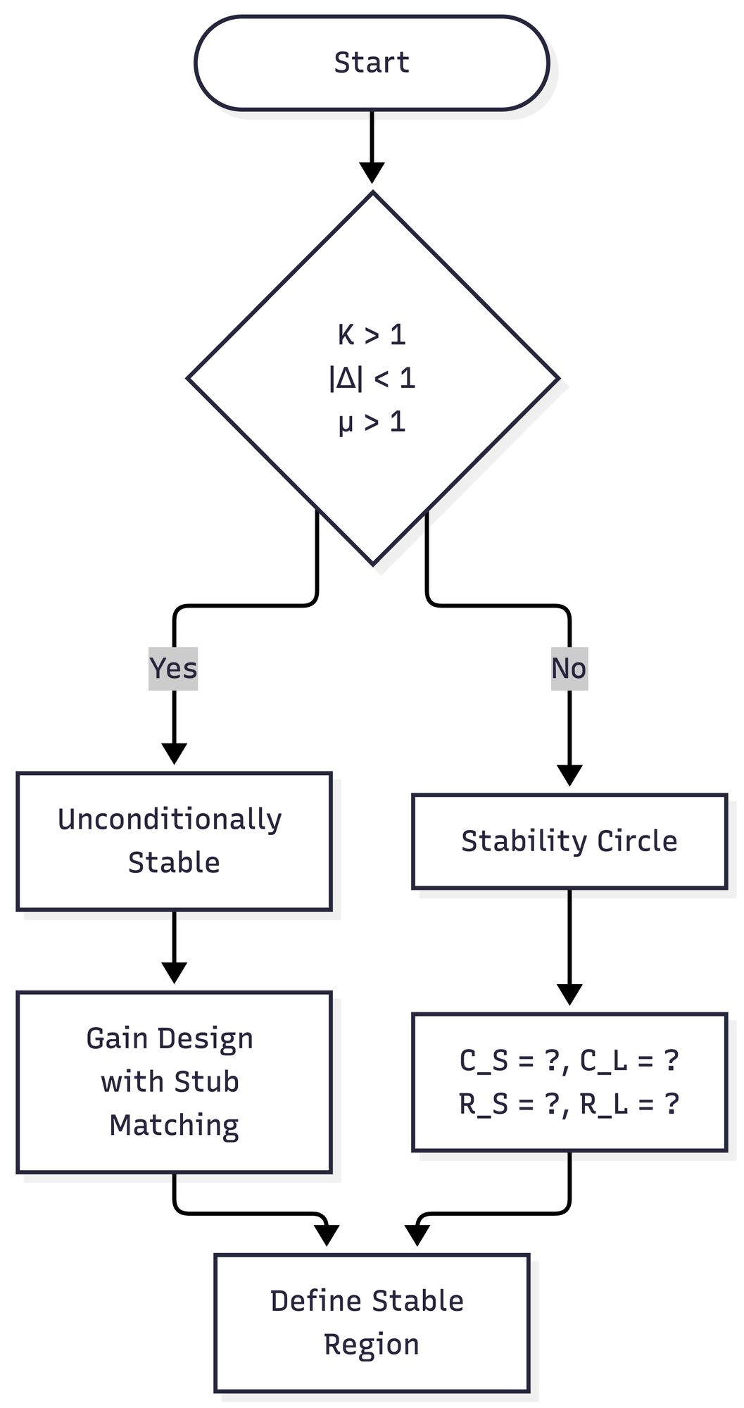
For a transistor that does not meet an unconditional-stability criterion, the stability-circle method provides the next level of analysis. Rather than concluding that the device cannot be used, the designer can determine the source and load reflection-coefficient regions that satisfy the required stability conditions. In this way, analytical stability tests and stability-circle analysis complement each other: the analytical tests provide a compact unconditional-stability check, while the stability circles provide detailed information about permissible terminations when stability depends on the selected source and load impedances.