Numerical 2 Stability Analysis

Before designing a microwave amplifier, it is essential to verify whether the transistor will operate stably for the intended source and load terminations. Stability analysis helps identify whether unwanted oscillations may occur and determines whether special care is required when designing the matching networks. In this example, the stability of a transistor operating at 800 MHz is investigated using the K-Δ stability criterion and stability-circle analysis.

her the transistor is unconditionally stable or conditionally stable and then evaluate the corresponding source and load stability circles.

2. Calculation of the S-Matrix Determinant

2.1 Determination of Δ

The determinant of the transistor S-matrix is given by:

\[ \Delta=S_{11}S_{22}-S_{12}S_{21} \]

Substituting the given S-parameters:

\[ \Delta=0.504\angle249.6^\circ \]

Therefore:

\[ |\Delta|=0.504 \]

The determinant magnitude is less than unity, satisfying one of the requirements for unconditional stability. However, the K-factor must also be evaluated before a final conclusion can be reached.

2.2 Physical Significance of Δ

The determinant Δ is an important parameter in microwave stability analysis because it combines the effects of input reflection, output reflection, forward gain, and reverse transmission into a single quantity. It appears directly in the equations for stability circles and unconditional stability tests. Although a value of |\Delta| less than unity is desirable, it does not by itself guarantee stability.

3. Calculation of Rollet Stability Factor (K-Factor)

3.1 K-Factor Formula

Rollet's stability factor is calculated from:

\[ K= \frac{ 1-|S_{11}|^2-|S_{22}|^2+|\Delta|^2 }{ 2|S_{12}S_{21}| } \]

Substituting the transistor S-parameters gives:

\[ K=0.547 \]

3.2 Interpretation of K

For unconditional stability, the transistor must satisfy:

\[ K>1 \]

\[ |\Delta|<1 \]

Although the determinant condition is satisfied, the calculated K-factor is less than unity. Therefore, the transistor does not satisfy the requirements for unconditional stability.

4. Stability Classification

4.1 Application of the K-Δ Criterion

The calculated values are:

\[ K=0.547 \]

\[ |\Delta|=0.504 \]

Comparing these values with the unconditional stability requirements:

\[ K<1 \]

\[ |\Delta|<1 \]

This corresponds to the conditionally stable case. The transistor is capable of stable operation, but only for certain source and load reflection coefficients. Some passive source and load impedances may still lead to instability.

4.2 Engineering Conclusion

Since the transistor is conditionally stable, the stable and unstable regions of the Smith Chart must be identified before designing the matching networks. Stability-circle analysis is therefore required.

5. Source Stability Circle

5.1 Source Stability Circle Center

The center of the source stability circle is:

\[ C_S=1.79\angle122^\circ \]

The location of this center in the complex reflection-coefficient plane determines the position of the source stability boundary on the Smith Chart.

5.2 Source Stability Circle Radius

The radius of the source stability circle is:

\[ R_S=1.04 \]

This radius defines the size of the source stability boundary. Together with the center location, it separates source reflection coefficients that produce stable operation from those that may result in oscillation.

5.3 Significance of the Source Stability Circle

The source stability circle is plotted on the source Smith Chart and represents the boundary where the magnitude of the output reflection coefficient becomes unity. One side of the circle corresponds to stable operation, while the opposite side corresponds to potentially unstable operation. A test point must be used to determine which side of the boundary is stable.

6. Load Stability Circle

6.1 Load Stability Circle Center

The center of the load stability circle is:

\[ C_L=1.3\angle48^\circ \]

This center specifies the location of the load stability boundary in the load reflection-coefficient plane.

6.2 Load Stability Circle Radius

The radius of the load stability circle is:

\[ R_L=0.45 \]

The radius determines the extent of the load stability boundary and helps identify permissible load reflection coefficients.

6.3 Significance of the Load Stability Circle

The load stability circle represents the boundary for which the magnitude of the input reflection coefficient becomes unity. Reflection coefficients lying on opposite sides of the circle correspond to stable and unstable operating regions. By plotting the circle on a Smith Chart and evaluating a suitable test point, the stable region can be identified.

7. Interpretation of the Stability Circles

Because the transistor is conditionally stable, the source and load stability circles play an important role in amplifier design. The matching networks must be designed so that the resulting source reflection coefficient \(\Gamma_S\) and load reflection coefficient \(\Gamma_L\) remain inside the stable regions. Failure to do so may cause oscillation even though the transistor is operating at the intended frequency.

The calculated values of \(C_S\), \(R_S\), \(C_L\), and \(R_L\) provide all the information required to construct the stability circles on the Smith Chart. Once plotted, the designer can determine the allowable source and load impedance regions and proceed with gain or noise optimization while maintaining stable operation.

Step 1: Measure the Smith Chart Radius 

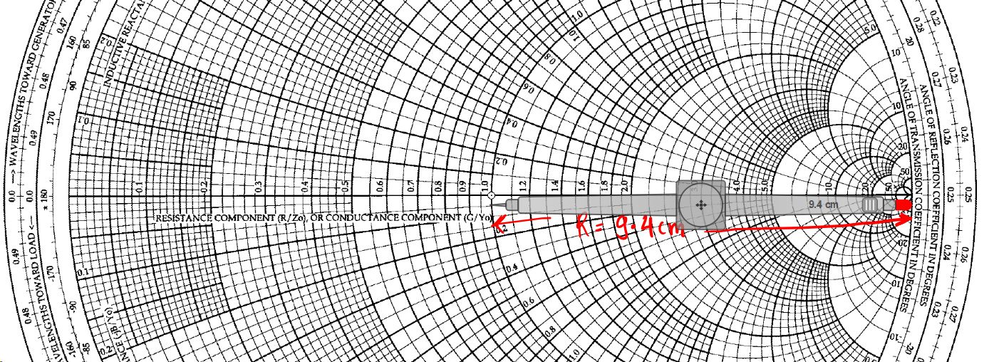
Measure the physical radius (r) of the Smith chart from the center to the outer perimeter using a ruler.

• Value: r = 9.4 cm

• Verification: Confirm the measurement matches the outer circumference zero-reflection point.

Step 2: Draw stability circle for source

Plot the Input Stability Circle (Source  Plane) (CS = 1.79∠122°  and RS =1.04):

• Angle Line: Draw a line from the center of the chart outward at an angle of 122° using the outer perimeter scale.

• Center Location: Compute the scaled distance for the source center (1.79 X 9.4 cm = 16.83 cm) and mark point Cs along the 122° line.

• Circle Radius: Compute the compass opening for the radius (1.04 X 9.4 cm = 9.78 cm).

• Draw Circle: Place the compass needle at point CS and draw the input stability circle.

• Verification: Check that both circle centers and radii match the calculated values from your design metrics.

Draw a line from the center of the Smith chart outward at an angle of 48° using the outer angle scale ("Angle of Reflection Coefficient in Degrees").

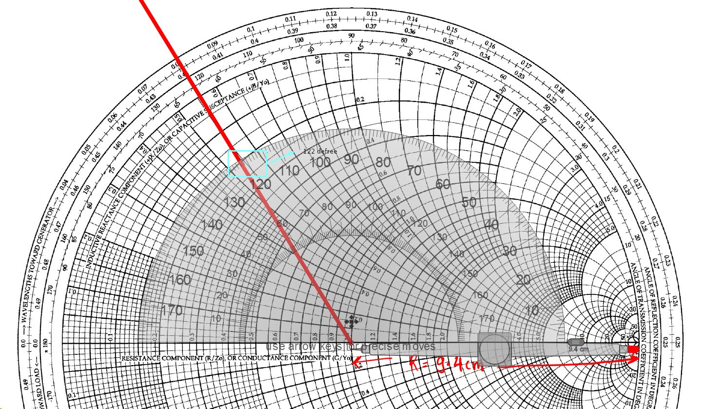
• Center Location: Compute the scaled distance for the source center (1.79 X 9.4 cm = 16.83 cm) and mark point Cs along the 122° line.

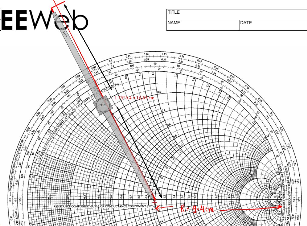
Circle Radius: Compute the compass opening for the radius (1.04 X 9.4 cm = 9.78 cm).

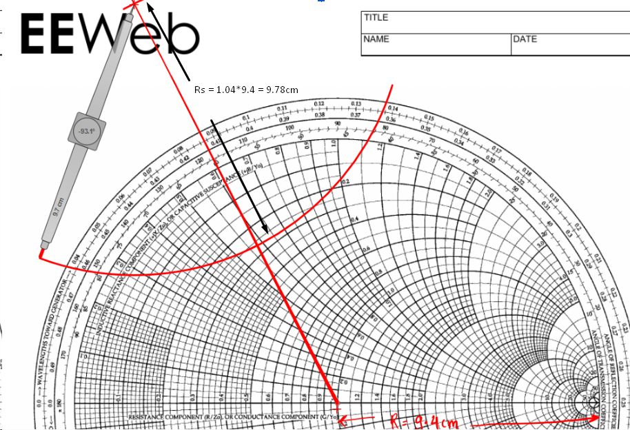
Step 3: Draw Stability circle for load too

Plot the Input Output Circle (Load Plane) 

Using the calculated output stability parameters (CL = 1.3∠48° and RL = 0.45):

• Angle Line: Draw a line from the center of the Smith chart outward at an angle of 48° using the outer angle scale ("Angle of Reflection Coefficient in Degrees").

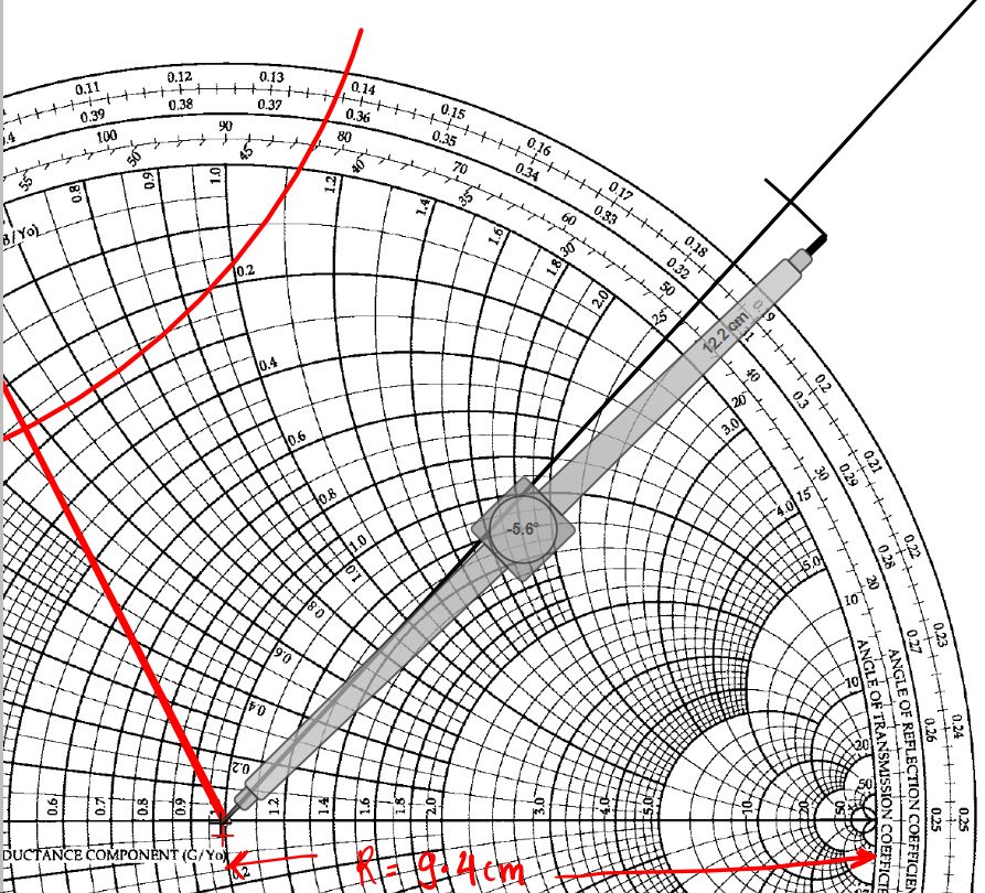
• Center Location: Multiply the magnitude of CL by the chart radius (1.3X9.4 cm = 12.22 cm) and mark the center point CL along the 48° line.

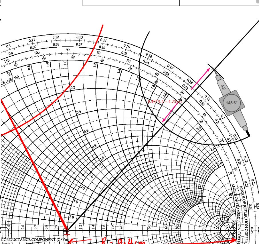
• Circle Radius: Calculate the compass opening for the radius (0.45 X 9.4 cm = 4.23cm).

• Draw Circle: Place the compass needle at point CL and draw the output stability circle with radius 4.23 cm.

• Verification: Ensure the circle intersects the proper regions of the Smith chart corresponding to the normalized impedance plane.

Plot value for radius CL = 1.3∠48° =1.3*9.4cm = 12.22 cm

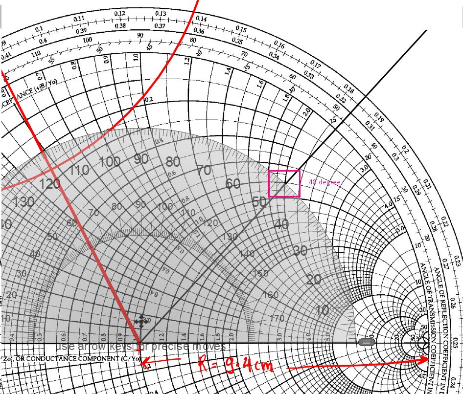
Center Location: Multiply the magnitude of CL by the chart radius (1.3X9.4 cm = 12.22 cm) and mark the center point CL along the 48° line.

Circle Radius: Calculate the compass opening for the radius (0.45 X 9.4 cm = 4.23cm).

Step 4: Define Stability Parameters according to conditions

Identify the safe operating regions by checking whether |S11| or |S22| is less than 1 to shade the permitted regions for ΓS and ΓL

Verification: Confirm that the stable load and source reflection coefficient areas are clearly marked outside or inside the respective circles based on the device's potential instability. 

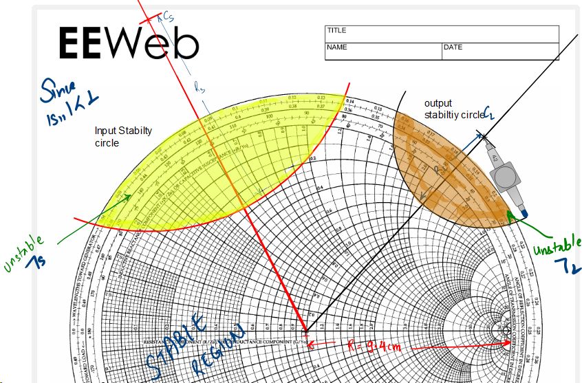
8. Final Stability Assessment

The determinant of the S-matrix was found to be:

\[ |\Delta|=0.504 \]

and the Rollet stability factor was calculated as:

\[ K=0.547 \]

Although |\Delta| is less than unity, the K-factor is less than one. Consequently, the transistor does not satisfy the unconditional stability criterion. The device is therefore classified as conditionally stable at 800 MHz.

Because the transistor is conditionally stable, stability-circle construction is necessary. The calculated source stability circle parameters \(C_S=1.79\angle122^\circ\) and \(R_S=1.04\), together with the load stability circle parameters \(C_L=1.3\angle48^\circ\) and \(R_L=0.45\), define the stability boundaries that must be considered when selecting source and load matching networks. By ensuring that the chosen reflection coefficients lie within the stable regions, the amplifier can operate without oscillation while achieving the desired performance objectives.