Numerical Microwave Amplifier Design at 5 GHz
S-Parameter Extraction & Stability Assessment at 5.0 GHz
The design of the microwave transistor amplifier from \(3.0\text{ GHz}\) to \(5.0\text{ GHz}\) begins with evaluating the active device's scattering parameters with respect to a reference characteristic impedance of \(Z_0 = 50\,\Omega\). The measured S-parameters across the frequency range are provided below:
\[ \begin{array}{c|c|c|c|c} f\,(\text{GHz}) & S_{11} & S_{12} & S_{21} & S_{22}\\ \hline 3.0 & 0.80\angle -89^\circ & 0.03\angle56^\circ & 2.86\angle99^\circ & 0.76\angle-41^\circ\\ 4.0 & 0.725\angle-116^\circ & 0.03\angle57^\circ & 2.60\angle76^\circ & 0.73\angle-54^\circ\\ 5.0 & 0.66\angle-142^\circ & 0.03\angle62^\circ & 2.39\angle54^\circ & 0.72\angle-68^\circ \end{array} \]
Focusing specifically on taking \(5.0\text{ GHz}\), the extracted parameters are mapped to calculator variables:
\(0.66\angle -142^\circ\)
\(0.03\angle 62^\circ\)
\(2.39\angle 54^\circ\)
\(0.72\angle -68^\circ\)
Before proceeding with conjugate matching, the stability is evaluated using the determinant \(\Delta\) and Rollet stability factor \(K\):
\[ \Delta = S_{11}S_{22} - S_{12}S_{21} = (0.66\angle -142^\circ)(0.72\angle -68^\circ) - (0.03\angle 62^\circ)(2.39\angle 54^\circ) \approx 0.418\angle 155.5^\circ \]
\[ K = \frac{1 - |S_{11}|^2 - |S_{22}|^2 + |\Delta|^2}{2 |S_{12} S_{21}|} = \frac{1 - (0.66)^2 - (0.72)^2 + (0.418)^2}{2(0.03)(2.39)} \approx 1.54 \]
Since \(K = 1.54 > 1\) and \(|\Delta| = 0.418 < 1\), the transistor is unconditionally stable at \(5.0\text{ GHz}\).
Calculator Trick & Workflow Hint:
- Set calculator to Complex Mode (Mode + 2).
- Assign inputs: Type magnitude, press Shift + (-) for \(\angle\), enter angle, then press Shift + STO + A (for \(S_{11}\)), B (\(S_{12}\)), C (\(S_{21}\)), and D (\(S_{22}\)).
- Compute determinant: Evaluate \(\mathbf{A}\mathbf{D} - \mathbf{B}\mathbf{C}\) and store magnitude into E via Shift + STO + E.
2. Stability Assessment & Determinant Calculation
To ensure the GaAs FET transistor can operate safely without oscillating under maximum gain conditions, we must verify its unconditional stability at \(5.0\text{ GHz}\). This requires calculating the scattering matrix determinant \(\Delta\) and the Rollet stability factor \(K\).
First, the determinant \(\Delta\) is calculated using the assigned variables (\(\mathbf{A}, \mathbf{B}, \mathbf{C}, \mathbf{D}\)):
\[ \Delta = S_{11}S_{22} - S_{12}S_{21} = \mathbf{A}\mathbf{D} - \mathbf{B}\mathbf{C} \]
\[ \Delta = (0.66\angle -142^\circ)(0.72\angle -68^\circ) - (0.03\angle 62^\circ)(2.39\angle 54^\circ) \]
\[ S_{11}S_{22} = (0.66 \times 0.72)\angle (-142^\circ + (-68^\circ)) = 0.4752\angle -210^\circ = 0.4752\angle 150^\circ \]
\[ S_{12}S_{21} = (0.03 \times 2.39)\angle (62^\circ + 54^\circ) = 0.0717\angle 116^\circ \]
\[ \Delta \approx 0.418\angle 155.5^\circ \implies |\Delta| \approx 0.418 \quad (\text{Store magnitude into } \mathbf{E}) \]
Next, we substitute these parameters into the Rollet stability factor equation:
\[ K = \frac{1 - |S_{11}|^2 - |S_{22}|^2 + |\Delta|^2}{2 |S_{12} S_{21}|} \]
\[ K = \frac{1 - (0.66)^2 - (0.72)^2 + (0.418)^2}{2(0.03)(2.39)} = \frac{1 - 0.4356 - 0.5184 + 0.1747}{0.1434} = \frac{0.2207}{0.1434} \approx 1.54 \]
Since the criteria for unconditional stability are \(K > 1\) and \(|\Delta| < 1\), and our calculated values are \(K = 1.54 > 1\) and \(|\Delta| = 0.418 < 1\), the transistor is confirmed to be unconditionally stable at \(5.0\text{ GHz}\).
Calculator Trick & Workflow Hint:
- Compute the determinant directly using memory slots: A × D - B × C.
- Isolate and store the determinant magnitude into variable E via Shift + STO + E for subsequent matching calculations.
- Evaluate \(K\) rapidly by inputting magnitudes squared using Shift + Hyp (Abs) for each term.
3: Intermediate Coefficients & Quadratic Parameters
To solve for the optimal source and load reflection coefficients (\(\Gamma_S, \Gamma_L\)) using simultaneous conjugate matching equations, we first need to compute several intermediate scalar and complex parameters. These include the scalar coefficients \(B_1\) and \(B_2\), and the complex matching coefficients \(C_1\) and \(C_2\).
The governing formulas for these parameters are defined as:
\[ B_1 = 1 + |S_{11}|^2 - |S_{22}|^2 - |\Delta|^2, \quad B_2 = 1 + |S_{22}|^2 - |S_{11}|^2 - |\Delta|^2 \]
\[ C_1 = S_{11} - \Delta S_{22}^*, \quad C_2 = S_{22} - \Delta S_{11}^* \]
Substituting the S-parameters and determinant magnitude (\(|\Delta| \approx 0.418\)) at \(5.0\text{ GHz}\):
1. Calculation of scalar \(B_1\):
\[ B_1 = 1 + (0.66)^2 - (0.72)^2 - (0.418)^2 = 1 + 0.4356 - 0.5184 - 0.1747 \approx 0.742 \quad (\text{Store into } \mathbf{F}) \]
2. Calculation of scalar \(B_2\):
\[ B_2 = 1 + (0.72)^2 - (0.66)^2 - (0.418)^2 = 1 + 0.5184 - 0.4356 - 0.1747 \approx 0.908 \quad (\text{Store into } \mathbf{X}) \]
3. Calculation of complex coefficient \(C_1\):
\[ C_1 = (0.66\angle -142^\circ) - (0.418\angle 155.5^\circ)(0.72\angle 68^\circ)^* \]
\[ C_1 = 0.66\angle -142^\circ - (0.418\angle 155.5^\circ)(0.72\angle -68^\circ) \approx 0.364\angle -146.5^\circ \quad (\text{Store into } \mathbf{Y}) \]
4. Calculation of complex coefficient \(C_2\):
\[ C_2 = (0.72\angle -68^\circ) - (0.418\angle 155.5^\circ)(0.66\angle -142^\circ)^* \]
\[ C_2 = 0.72\angle -68^\circ - (0.418\angle 155.5^\circ)(0.66\angle 142^\circ) \approx 0.446\angle -71.4^\circ \quad (\text{Store into } \mathbf{M}) \]
Calculator Trick & Workflow Hint:
- Use absolute value function Shift + Hyp (Abs) for magnitude squared expressions like \(\text{Abs}(\mathbf{A})^2\).
- Access complex conjugate via Shift + 2, then select option 2 (\(\mathrm{conj}\)) for complex variables.
- Store intermediate outputs into memory slots F, X, Y, and M to streamline the final root calculations in Part 4.
4: Optimal Reflection Coefficients (\(\Gamma_S, \Gamma_L\)) Selection & Stub Matching Layout
With the intermediate scalar and complex parameters successfully computed and stored in memory variables (\(\mathbf{F}, \mathbf{X}, \mathbf{Y}, \mathbf{M}\)), we now apply the quadratic formula branches to solve for the optimal source and load reflection coefficients (\(\Gamma_S, \Gamma_L\)). For passive stability, we select the physically realizable roots where magnitudes are strictly less than 1 (\(|\Gamma_S| < 1\) and \(|\Gamma_L| < 1\)).
The general quadratic formulas for the reflection coefficients are:
\[ \Gamma_S = \frac{B_1 \pm \sqrt{B_1^2 - 4 |C_1|^2}}{2 C_1}, \quad \Gamma_L = \frac{B_2 \pm \sqrt{B_2^2 - 4 |C_2|^2}}{2 C_2} \]
1. Calculation of Source Reflection Coefficient (\(\Gamma_S\)):
\[ \Gamma_S = \frac{0.742 - \sqrt{(0.742)^2 - 4(0.364)^2}}{2(0.364\angle -146.5^\circ)} \]
\[ \Gamma_S = \frac{0.742 - \sqrt{0.5506 - 0.5300}}{0.728\angle -146.5^\circ} = \frac{0.742 - 0.1435}{0.728\angle -146.5^\circ} = \frac{0.5985}{0.728\angle -146.5^\circ} \approx 0.78\angle 146.5^\circ \]
2. Calculation of Load Reflection Coefficient (\(\Gamma_L\)):
\[ \Gamma_L = \frac{0.908 - \sqrt{(0.908)^2 - 4(0.446)^2}}{2(0.446\angle -71.4^\circ)} \]
\[ \Gamma_L = \frac{0.908 - \sqrt{0.8245 - 0.7957}}{0.892\angle -71.4^\circ} = \frac{0.908 - 0.1697}{0.892\angle -71.4^\circ} = \frac{0.7383}{0.892\angle -71.4^\circ} \approx 0.828\angle 71.4^\circ \]
3. Stub Matching Network Layout:
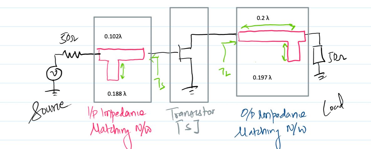
Using the derived optimal reflection coefficients \(\Gamma_S = 0.78\angle 146.5^\circ\) and \(\Gamma_L = 0.828\angle 71.4^\circ\), the input and output matching networks are realized via single-stub or double-stub configurations on a Smith Chart relative to the \(50\,\Omega\) reference characteristic impedance, completing the maximum gain amplifier design at \(5.0\text{ GHz}\).]
5. Gain Calculations
With the stability factor \(K = 1.54\) verified and the optimal reflection coefficients (\(\Gamma_S, \Gamma_L\)) determined at \(5.0\text{ GHz}\), we now evaluate the power gain of the amplifier. Because the transistor is bilateral (\(S_{12} \neq 0\)), we calculate both the rigorous Bilateral Maximum Available Gain (MAG) using the Rollet stability factor \(K\), the Transducer Power Gain via individual gain factors, and compare it with the Unilateral Gain Approximation to quantify reverse isolation effects.
1. Bilateral Maximum Available Gain (MAG) using Stability Factor \(K\):
Since the device is unconditionally stable (\(K = 1.54 > 1\)), the maximum available power gain is given by the classic bilateral formula:
\[ MAG = \frac{|S_{21}|}{|S_{12}|} \left( K - \sqrt{K^2 - 1} \right) \]
\[ MAG = \frac{2.39}{0.03} \left( 1.54 - \sqrt{(1.54)^2 - 1} \right) = 79.67 \left( 1.54 - \sqrt{2.3716 - 1} \right) \]
\[ MAG = 79.67 \left( 1.54 - \sqrt{1.3716} \right) = 79.67 \left( 1.54 - 1.1711 \right) = 79.67 \times 0.3689 \approx 29.39 \]
\[ MAG_{\mathrm{dB}} = 10 \log_{10}(29.39) \approx 14.68\text{ dB} \]
2. Transducer Power Gain via Individual Effective Gain Factors:
Alternatively, the total transducer power gain can be verified by multiplying the individual linear gain contributions of the input network (\(G_S\)), the active device (\(G_0\)), and the output network (\(G_L\)):
\[ G_S = \frac{1}{1 - |\Gamma_S|^2} = \frac{1}{1 - (0.78)^2} = \frac{1}{1 - 0.6084} = \frac{1}{0.3916} \approx 2.553 \quad (4.07\text{ dB}) \]
\[ G_0 = |S_{21}|^2 = (2.39)^2 \approx 5.712 \quad (7.57\text{ dB}) \]
\[ G_L = \frac{1 - |\Gamma_L|^2}{|1 - S_{22}\Gamma_L|^2} = \frac{1 - (0.828)^2}{|1 - (0.72\angle -68^\circ)(0.828\angle 71.4^\circ)|^2} \approx 2.016 \quad (3.04\text{ dB}) \]
\[ G_{T\max,\mathrm{dB}} = G_{S,\mathrm{dB}} + G_{0,\mathrm{dB}} + G_{L,\mathrm{dB}} = 4.07\text{ dB} + 7.57\text{ dB} + 3.04\text{ dB} = 14.68\text{ dB} \]
3. Unilateral Gain Approximation and Figure of Merit (\(U\)):
If reverse transmission is ignored (\(S_{12} = 0\)), the Maximum Unilateral Gain (\(G_{umax}\)) is calculated as:
\[ G_{umax} = \frac{1}{1 - |S_{11}|^2} |S_{21}|^2 \frac{1}{1 - |S_{22}|^2} = \frac{1}{1 - 0.66^2} (2.39)^2 \frac{1}{1 - 0.72^2} \]
\[ G_{umax} = 1.772 \times 5.712 \times 2.076 \approx 21.01 \implies 13.22\text{ dB} \]
To measure the error of this unilateral assumption, we compute the unilateral figure of merit \(U\):
\[ U = \frac{|S_{11}||S_{12}||S_{21}||S_{22}|}{(1 - |S_{11}|^2)(1 - |S_{22}|^2)} = \frac{0.66 \times 0.03 \times 2.39 \times 0.72}{(1 - 0.66^2)(1 - 0.72^2)} = \frac{0.0341}{0.2718} \approx 0.125 \]
The true bilateral gain is bounded by the unilateral error limits: \(\frac{1}{(1+U)^2} \le \frac{G_T}{G_{TU}} \le \frac{1}{(1-U)^2}\), confirming that bilateral matching is required for precise design.