Justification 

In high-frequency transmission line design, Shunt Stub Matching is used to match an arbitrary load impedance to the characteristic impedance of the transmission line. The technique employs a short-circuited or open-circuited stub connected in parallel with the main line to achieve impedance matching and maximum power transfer.

Understanding the physical and theoretical reasoning behind each design step helps engineers apply the method correctly and interpret Smith Chart movements more effectively.

Physical and Network Justification

Why Parallel (Shunt) Placement Uses Admittance

A shunt stub is connected in parallel with the transmission line. In a parallel network, admittances combine directly, making admittance the most convenient quantity for analysis.

The total input admittance at the junction is:

\[
y_{in} = y_d + y_{stub}
\]

Since admittances add directly in parallel circuits, calculations become much simpler when performed using admittance rather than impedance.

For this reason, the Smith Chart design procedure begins with the normalized admittance point rather than the normalized impedance point.

The normalized admittance is obtained from:

\[
y_N = \frac{1}{z_N}
\]

This admittance point serves as the primary reference throughout the matching procedure.

Why Short-Circuited Stubs Are Preferred Over Open-Circuited Stubs

Short-circuited stubs are generally preferred in practical microwave and RF systems for several important reasons.

First, shorted stubs are easier to construct accurately and adjust during implementation.

Second, open-circuited stubs tend to radiate electromagnetic energy from the open end, particularly at high frequencies. This unwanted radiation can cause power loss and may introduce interference within nearby circuits.

A short-circuited stub minimizes radiation and therefore provides better overall performance in most applications.

Step-by-Step Methodological Justification

Step 1: Load Normalization

The first step is to convert the actual load impedance into a normalized value.

The normalized impedance is:

\[
z_N = \frac{Z_L}{Z_0}
\]

Normalization converts specific impedance values into dimensionless quantities that can be plotted on a universal Smith Chart.

Because the Smith Chart is normalized, it can be used for any transmission line regardless of its characteristic impedance.

This process eliminates the need to create separate charts for different transmission line systems.

Step 4: Load Line Inversion (Impedance to Admittance Conversion)

After plotting the normalized impedance, the next step is to determine the corresponding normalized admittance.

This is accomplished by rotating through:

\[
180^\circ
\]

along the constant SWR circle.

The resulting point is the normalized admittance:

\[
y_N = \frac{1}{z_N}
\]

often identified as Point B on the Smith Chart.

This conversion is mandatory because the matching stub is connected in parallel with the transmission line.

Since parallel elements are analyzed using admittance, the matching process must begin from the admittance point rather than the impedance point.

Step 5: Moving to the \(R = 1\) Circle

The objective of shunt stub matching is to locate a point on the transmission line where the real component of the normalized admittance equals unity.

This condition is represented by:

\[
g = 1
\]

Moving clockwise along the SWR circle eventually reaches the unity conductance circle.

At this location the normalized admittance becomes:

\[
y_d = 1 + jb_n
\]

The real part is now perfectly matched to the characteristic admittance of the transmission line.

During denormalization:

\[
Y = yY_0
\]

the real component becomes:

\[
Y = Y_0
\]

which corresponds to a matched condition.

Only the reactive component remains to be corrected.

Steps 6 and 7: Wavelength Distance to Stub

Clockwise movement on the Smith Chart corresponds to movement from the load toward the generator.

The wavelength distance between the load admittance point and the unity conductance point determines the physical location where the stub must be connected.

The stub distance is calculated as:

\[
d_s = \text{WTG}_C - \text{WTG}_B
\]

If the result is negative, add:

\[
0.5\lambda
\]

to obtain the correct positive distance.

This measured distance represents the exact location on the transmission line where the real part of the admittance is already matched.

Step 8: Reactive Component Cancellation

At the selected location, the normalized admittance is:

\[
y_d = 1 + jb_n
\]

Although the real component is matched, the reactive component still exists.

To achieve a perfect match, the stub must introduce an equal susceptance with opposite polarity.

The required stub susceptance is:

\[
b_{stub} = -jb_n
\]

When the stub is connected in parallel, the total admittance becomes:

\[
y_{in} = y_d + y_{stub}
\]

Substituting the values gives:

\[
y_{in} = (1 + jb_n) + (-jb_n)
\]

which simplifies to:

\[
y_{in} = 1 + j0
\]

This represents a completely matched transmission line.

Step 9: Stub Length Calculation

After determining the required susceptance, the corresponding stub length must be found.

The length is measured along the perimeter of the Smith Chart on the:

\[
R = 0
\]

circle.

The starting point depends on the type of stub being used.

For a Short-Circuited Stub

Measurement begins at the infinite admittance point:

\[
y = \infty
\]

which is located at the rightmost point on the real axis.

The measured distance to the desired susceptance location determines the shorted stub length.

For an Open-Circuited Stub

Measurement begins at the zero admittance point:

\[
y = 0
\]

which is located at the leftmost point on the real axis.

The measured distance to the desired susceptance location determines the open stub length.

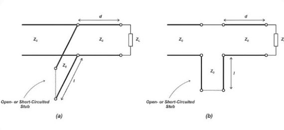
Shunt Stub Matching relies on admittance analysis because the matching element is connected in parallel with the transmission line. Normalization allows universal Smith Chart usage, admittance conversion establishes the proper reference point, movement to the unity conductance circle ensures resistive matching, wavelength measurements determine the stub location, and susceptance cancellation removes the reactive component. Together, these steps provide a systematic and physically meaningful method for achieving impedance matching in RF and microwave transmission systems.