Single-Stub Shunt Matching Explained

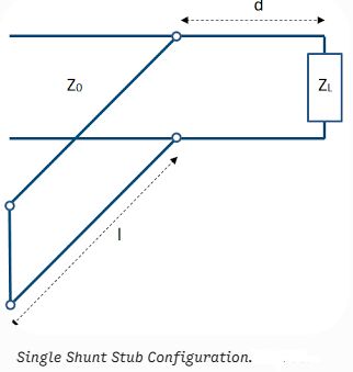
Single-Stub Shunt Matching is a widely used impedance matching technique in RF and microwave engineering. It employs a short-circuited or open-circuited transmission line stub connected in parallel with the main transmission line at a specific distance from the load. The purpose is to transform an arbitrary load impedance into a matched condition, minimizing reflections and maximizing power transfer.

Since the matching element is connected in parallel, admittance is more convenient than impedance for analysis. Engineers can design a shunt stub matching network using either analytical equations or the graphical Smith Chart method.

Understanding Single-Stub Shunt Matching
single-stub-shunt-matching-explained

A shunt stub is connected in parallel with the transmission line at a carefully selected location. The stub introduces a reactive admittance that cancels the unwanted susceptance present at that point on the line.

The normalized admittance is:

\[
y = \frac{Y}{Y_0} = g + jb
\]

where

\[
Y_0 = \frac{1}{Z_0}
\]

The objective is to achieve a matched condition:

\[
y_{in} = y_d + y_{stub} = 1 + j0
\]

When this condition is satisfied, the transmission line is perfectly matched.

Analytical Design Procedure

Step 1: Calculate the Normalized Load Admittance

Begin by converting the load impedance into normalized admittance.

\[
y_L = \frac{1}{z_L} = \frac{Z_0}{Z_L} = g_L + jb_L
\]

This value serves as the starting point for all subsequent calculations.

Step 2: Determine the Distance to the Stub

Move along the transmission line until the real part of the normalized admittance becomes unity.

The admittance transformation equation for a lossless transmission line is:

\[
y(d) = \frac{y_L + j\tan(\beta d)}
{1 + jy_L\tan(\beta d)}
\]

The matching condition requires:

\[
\text{Re}\{y(d)\} = 1
\]

which gives:

\[
y(d) = 1 + jb
\]

Solving this equation produces two valid solutions:

\[
d_1 \quad \text{and} \quad d_2
\]

within:

\[
0 \le d < \frac{\lambda}{2}
\]

Step 3: Determine the Required Stub Susceptance

At the chosen location, the transformed admittance becomes:

\[
y_d = 1 + jb
\]

To achieve a match, the stub must cancel the reactive component:

\[
b_{stub} = -b
\]

The total admittance then becomes:

\[
y_{in} = 1 + j0
\]

Step 4: Calculate the Stub Length

The required length depends on the type of stub used.

Short-Circuited Stub

The normalized admittance of a short-circuited stub is:

\[
y_{stub} = -j\cot(\beta l)
\]

Since:

\[
y_{stub} = -jb
\]

the required length is obtained from:

\[
\tan(\beta l) = \frac{1}{b}
\]

Open-Circuited Stub

The normalized admittance of an open-circuited stub is:

\[
y_{stub} = j\tan(\beta l)
\]

Since:

\[
y_{stub} = -jb
\]

the required length is determined from:

\[
\tan(\beta l) = -b
\]

The final solution must satisfy:

\[
0 \le l < \frac{\lambda}{2}
\]

If the calculated value is negative, add:

\[
\frac{\lambda}{2}
\]

Smith Chart Graphical Procedure for Shunt Stub Matching

When using a Smith Chart, all operations are performed in terms of admittance because the stub is connected in parallel.

Step 1: Normalize the Load Impedance

Calculate the normalized load impedance:

\[
z_N = \frac{Z_L}{Z_0}
\]

Step 2: Plot the Normalized Impedance

Locate the normalized impedance on the Smith Chart using the appropriate resistance circle and reactance arc.

Step 3: Draw the SWR Circle

Draw the SWR circle using the chart center as the pivot point.

The Standing Wave Ratio is read from the positive real axis:

\[
\text{SWR}
\]

Step 4: Find the Normalized Admittance (Point B)

Rotate the impedance point by 180 degrees around the chart center.

The normalized admittance becomes:

\[
y_N = \frac{1}{z_N}
\]

Record the wavelength reading:

\[
\text{WTG}_B
\]

Step 5: Move to the Unity Conductance Circle (Point C)

Move clockwise along the SWR circle until reaching the first intersection with the unity conductance circle.

At Point C:

\[
y_C = 1 + jb_n
\]

Step 6: Record the Wavelength Reading

Project Point C to the wavelength scale and record:

\[
\text{WTG}_C
\]

Step 7: Calculate the Distance to the Stub

The distance from the load to the stub connection point is:

\[
d_s = \text{WTG}_C - \text{WTG}_B
\]

If:

\[
\text{WTG}_C < \text{WTG}_B
\]

add:

\[
0.5\lambda
\]

Step 8: Determine the Required Stub Susceptance (Point D)

The susceptance at Point C is:

\[
+jb_n
\]

The stub must provide:

\[
b_{stub} = -jb_n
\]

Record the wavelength reading:

\[
\text{WTG}_D
\]

Step 9: Calculate the Stub Length

Short-Circuited Stub Length

Measure clockwise from the short-circuit point:

\[
l_s = \text{WTG}_D - 0.25\lambda
\]

If the result is negative, add:

\[
0.5\lambda
\]

Open-Circuited Stub Length

Measure clockwise from the open-circuit point:

\[
l_o = \text{WTG}_D
\]

Analytical Method vs Smith Chart Method Comparison  

Parameter Symbol / Variable Value
Normalized Load \(z_N\) \(Z_L / Z_0\)
Standing Wave Ratio \(\text{SWR}\) Read on Real Axis
Normalized Admittance (Point B) \(y_N\) \(1/z_N\)
Admittance WTG Reading \(\text{WTG}_B\) \(\text{?}\lambda\)
Matched Admittance (Point C) \(y_C\) \(1 + jb_n\)
Point C WTG Reading \(\text{WTG}_C\) \(\text{?}\lambda\)
Distance to Stub \(d_s\) \(\text{WTG}_C - \text{WTG}_B\)
Target Stub Susceptance \(b_{stub}\) \(-jb_n\)
Point D WTG Reading \(\text{WTG}_D\) \(\text{?}\lambda\)
Shorted Stub Length \(l_s\) \(\text{WTG}_D - 0.25\lambda\)
Open Stub Length \(l_o\) \(\text{WTG}_D\)